
![]()
Distributed Database Patterns
The manager is to be blamed who distributes parts to his players which they are unable to act.
—Franz Schubert
The speed of communications is wondrous to behold. It is also true that speed can multiply the distribution of information that we know to be untrue.
—Edward R. Murrow
Administrators of web applications have traditionally had two choices when the application demand exceeds database capacity: scaling up by increasing the power of individual servers, or scaling out by adding more servers. For most of the relational database era, scaling up was the more practical option. Early relational databases did not provide a clustering option, whereas the CPU and memory supplied by a single server was constantly and exponentially increasing in line with Moore’s law. Consequently, scaling out was neither practical nor necessary.
However, as database workloads shifted from client-server applications running behind the firewall to web applications with potentially global scope, it became increasingly difficult to support workload and availability requirements on a single server. Furthermore, Internet applications were often subject to unpredictable and massive growth in workload: it became possible for an application to “go viral” and to suddenly experience exponential growth in demand. The economic sweet spot for computer hardware and the imperatives of growth increasingly encouraged clusters of servers rather than single, monolithic proprietary servers. A scale-out solution for databases became imperative.
To address the demands of web-scale applications, a new generation of distributed nonrelational databases emerged. In this chapter, we’ll dive deep into the architectures of these distributed database systems.
Distributed Relational Databases
The first database systems were designed to run on a single computer. Indeed, prior to the client-server revolution, all components of early database applications—including all the application code—would reside on a single system: the mainframe.
In this centralized model, all program code runs on the server, and users communicate with the application code through dumb terminals (the terminals are “dumb” because they contain no application code). In the client-server model, presentation and business logic were implemented on workstations—usually Windows PCs—that communicated with a single back-end database server. In early Internet applications, business logic was implemented on one or more web application servers, while presentation logic was shared between the web browser and the application server, which still almost always communicated with a single database server.
Figure 8-1 Illustrates the three architectures, showing how each pattern continued to rely on a single, monolithic database server.

Figure 8-1. Mainframe, client-server, and early web architectures relied on single, monolithic database servers
Database replication was initially adopted as a means of achieving high availability. Using replication, database administrators could configure a standby database that could take over for the primary database in the event of failure.
Database replication often took advantage of the transaction log that most relational databases used to support ACID transactions. We introduced the transaction log pattern in the context of in-memory databases in Chapter 7. When a transaction commits in an ACID-compliant database, the transaction record is immediately written to the transaction log so that it is preserved in the event of failure. A replication process monitoring the transaction log can apply changes to a backup database, thereby creating a replica.
Figure 8-2 illustrates the log-based replication approach. Database transactions are written in an asynchronous “lazy” manner to the database files (1), but a database transaction immediately writes to the transaction log upon commit (2). The replication process monitors the transaction log and applies transactions as they are written to the read-only slave database (3). Replication is usually asynchronous, but in some databases the commit can be deferred until the transaction has been replicated to the slave.

Figure 8-2. Log-based replication
As we saw in Chapter 3, replication is typically a first step toward distributing the database load across multiple servers. Using replication, the read workload can be distributed in a scale-out fashion, although database transactions must still be applied to the master copy.
Shared Nothing and Shared Disk
The replication pattern for distributing database workloads works well to distribute read activity across multiple servers, but it does not distribute transactional write loads, which still must be directed exclusively to the master server.
Replication is also of limited value for distributing data warehousing workloads. An OLTP workload typically consists of large numbers of short-duration requests. However, in a data warehousing environment, the workload usually consists of smaller numbers of data-intensive queries. In high-end database servers, these massive queries are executed by multiple processes or threads, each of which can leverage a separate CPU core and take advantage of multiple IO channels.
Parallelizing a query across multiple database servers requires a new approach. Data warehousing vendors provided a solution to this problem by implementing a shared-nothing clustered database architecture. Like so many concepts in the relational world, the shared-nothing idea was most notably outlined by Michael Stonebraker in the 1980s. A database server may be classified as:
- Shared-everything: In this case, every database process shares the same memory, CPU, and disk resources. Sharing memory implies that every process is on the same server and hence this architecture is a single-node database architecture.
- Shared-disk: In this case, database processes may exist on separate nodes in the cluster and have access to the CPU and memory of the server on which they reside. However, every process has equal access to disk devices, which are shared across all nodes of the cluster.
- Shared-nothing: In this case, each node in the cluster has access not only to its own memory and CPU but also to dedicated disk devices and its own subset of the database. We’ve seen several examples of shared-nothing architecture in this book already, including the sharded MySQL design in Chapter 3 and the VoltDB partitioning scheme in Chapter 7.
The shared-nothing model became the basis for several early clustered database systems, such as Teradata. It provides an attractive model for data warehousing workloads because queries can easily be parallelized across the multiple nodes based on the data they wish to access. For a system that wishes to maximize read-centric workloads, it is significantly easier to implement. Databases implementing the shared-nothing model often refer to themselves as massively parallel processing (MPP) databases. Figure 8-3 illustrates the shared-nothing model.
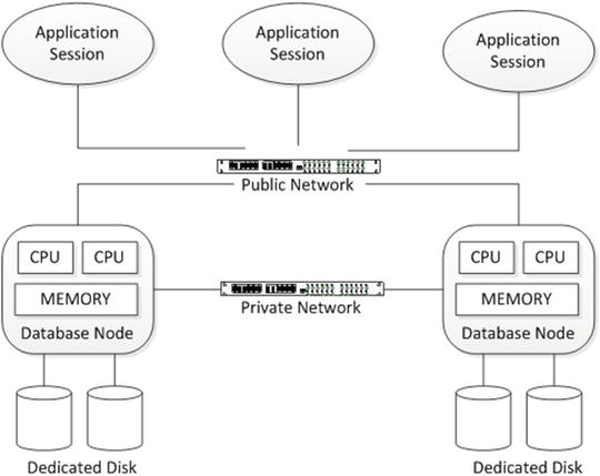
Figure 8-3. Shared-nothing database architecture
The shared-nothing architecture tends to break down in transactional scenarios, because of the need to coordinate transactions that may touch data on multiple nodes. Since ACID transactions are “all or nothing,” it’s necessary for all nodes in the transaction to coordinate closely on transaction execution. This coordination, known as two-phase commit, is notoriously difficult to implement and may result in “in doubt” transactional outcomes and poor transactional performance.
The other drawback of the shared-nothing architecture is that without careful partitioning, the cluster workload becomes unbalanced. Maintaining correct partitioning becomes a major operational activity. When nodes are added or removed from the cluster, expensive rebalancing is required.
A shared-disk architecture theoretically allows for greater and more elastic scalability, and it removes the need for rebalancing operations. It also provides a more economical high-availability solution, since no node has exclusive responsibility for any particular set of data. In shared-nothing, a node failure results in a portion of the database being unavailable, while in shared-disk, the remaining nodes are able to take over responsibility for the failed node.
The challenge for the shared-disk architecture is the need to coordinate cached data across nodes. Without an in-memory cache, performance for all operations will degrade to disk speed. But to maintain a consistent view of data across all nodes, each node needs to maintain a consistent cache. Maintaining this cache coherency puts a strain on the network between the nodes and is difficult to successfully implement.
To date, the only surviving commercially successful shared-disk RDBMS is Oracle’s Real Application Clusters (RAC) cluster database. RAC is the basis for Oracle’s Exadata database machine and cloud database offerings. Figure 8-4 illustrates the shared-disk model.

Figure 8-4. Shared-disk database architecture
Nonrelational Distributed Databases
Maintaining ACID transactional integrity across multiple nodes in a distributed relational database is a significant challenge. However, in nonrelational database systems, ACID compliance is often not provided. For nonrelational distributed databases, the following considerations become more significant:
- Balancing availability and consistency: As we saw in Chapter 3, Brewer’s CAP theorem argues that a distributed database that aims to scale beyond a single local network must choose between availability and consistency in the event of a network partition. An ACID-compliant database is obliged to favor consistency over all other factors. However, a nonrelational database without the constraint of strict ACID compliance can strike a different balance.
- Hardware economics: Even small differences in the cost of individual servers multiply quickly when a system scales to thousands or hundreds of thousands of nodes. Therefore, an economical database architecture will better leverage commodity hardware so as to take advantage of the best price/performance ratios available. Furthermore, it may become necessary to be able to cope with disparities between server configurations, so that new hardware can be added to the database cluster without requiring all existing nodes to be upgraded to the latest hardware specification.
- Resilience:In a massive database cluster, nodes will fail from time to time. In the event of these failures, there can be no data loss, interruption to availability, or maybe even failure at the transaction level.
There have been three broad categories of distributed database architecture adopted by next-generation databases. The three models are:
- Variations on traditional sharding architecture, in which data is segmented across nodes based on the value of a “shard key.”
- Variations on the Hadoop HDFS/HBase model, in which an “omniscient master” determines where data should be located in the cluster, based on load and other factors
- The Amazon Dynamo consistent hashing model, in which data is distributed across nodes of the cluster based on predictable mathematical hashing of a key value.
Replication may be inherent within each of these architectures in order to ensure that no data is lost in the event of a server failure, although the replication strategies vary. We look at examples of each of these approaches in the remainder of this chapter. We use MongoDB as an example of a sharding architecture, HBase as the example of an omniscient master, and Cassandra as an example of Dynamo-style consistent hashing.
MongoDB Sharding and Replication
MongoDB supports sharding to provide scale-out capabilities and replication for high availability. Although each can be implemented independently of the other, they are usually both present in a production scenario.
Sharding
A high-level representation of the MongoDB sharding architecture is shown in Figure 8-5. Each shard is implemented by a distinct MongoDB database, which in most respects is unaware of its role in the broader sharded server (1). A separate MongoDB database—the config server (2)—contains the metadata that can be used to determine how data is distributed across shards. A router process (3) is responsible for routing requests to the appropriate shard server.
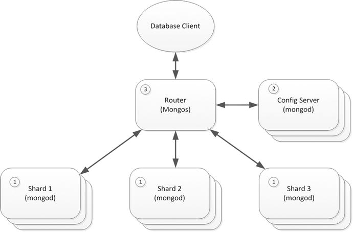
Figure 8-5. MongoDB sharding architecture
You may recall that in MongoDB, a collection is used to store multiple JSON documents that usually have some common attributes. To shard a collection, we choose a shard key, which is one or more indexed attributes that will be used to determine the distribution of documents across shards. The B-tree structure of the MongoDB index contains the information necessary to distribute keys evenly across shards.
Distribution of data across shards can be either range based or hash based. In range-based partitioning, each shard is allocated a specific range of shard key values. MongoDB consults the distribution of key values in the index to ensure that each shard is allocated approximately the same number of keys. In hash-based sharding, the keys are distributed based on a hash function applied to the shard key.
There are advantages and compromises involved in each scheme. Figure 8-6 illustrates the performance trade-offs inherent in range and hash sharding for inserts and range queries.

Figure 8-6. Comparison of range and hash sharding in MongoDB
Range-based partitioning allows for more efficient execution of queries that process ranges of values, since these queries can often be resolved by accessing a single shard. Hash-based sharding requires that range queries be resolved by accessing all shards. On the other hand, hash-based sharding is more likely to distribute “hot” documents (unfilled orders or recent posts, for instance) evenly across the cluster, thus balancing the load more effectively.
However, when range partitioning is enabled and the shard key is continuously incrementing, the load tends to aggregate against only one of the shards, thus unbalancing the cluster. With hash-based partitioning new documents are distributed evenly across all members of the cluster. Furthermore, although MongoDB tries to distribute shard keys evenly across the cluster, it may be that there are hotspots within particular shard key ranges which again unbalance the load. Hash-based sharding is more likely to evenly distribute the load in this scenario.
Tag-aware sharding allows the MongoDB administrator to fine-tune the distribution of documents to shards. By associating a shard with the tag, and associating a range of keys within a collection with the same tag, the administrator can explicitly determine the shard on which these documents will reside. This can be used to archive data to shards on cheaper, slower storage or to direct particular data to a specific data center or geography.
When hash-based sharding is implemented, the number of documents in each shard tends to remain balanced in most scenarios. However, in a range-based sharding scenario, it is easy for the shards to become unbalanced, especially if the shard key is based on a continuously increasing value, such as an auto-incrementing primary key ID.
For this reason, MongoDB will periodically assess the balance of shards across the cluster and perform rebalance operations, if needed. The unit of rebalance is the shard chunk. Shards consist of chunks—typically 64MB in size—that contain contiguous values of shard keys (or of hashed shard keys). If a shard is added or removed from the cluster, or if the balancer determines that a shard has become unbalanced, it can move chunks from one shard to another. The chunks themselves will be split if they grow too large.
Sharding is almost always combined with replication so as to ensure both availability and scalability in a production MongoDB deployment.
In MongoDB, data can be replicated across machines by the means of replica sets. A replica set consists of a primary node together with two or more secondary nodes. The primary node accepts all write requests, which are propagated asynchronously to the secondary nodes.
The primary node is determined by an election involving all available nodes. To be eligible to become primary, a node must be able to contact more than half of the replica set. This ensures that if a network partitions a replica set in two, only one of the partitions will attempt to establish a primary.
The successful primary will be elected based on the number of nodes to which it is in contact, together with a priority value that may be assigned by the system administrator. Setting a priority of 0 to an instance prevents it from ever being elected as primary. In the event of a tie, the server with the most recent optime—the timestamp of the last operation—will be selected.
The primary stores information about document changes in a collection within its local database, called the oplog. The primary will continuously attempt to apply these changes to secondary instances.
Members within a replica set communicate frequently via heartbeat messages. If a primary finds it is unable to receive heartbeat messages from more than half of the secondaries, then it will renounce its primary status and a new election will be called. Figure 8-7 illustrates a three-member replica set and shows how a network partition leads to a change of primary.

Figure 8-7. MongoDB replica set and primary failover
Arbiters are special servers that can vote in the primary election, but that don’t hold data. For large databases, these arbiters can avoid the necessity of creating otherwise unnecessary extra servers to ensure that a quorum is available when electing a primary.
Write Concern and Read Preference
A MongoDB application has some control over the behavior of read and write operations, providing a degree of tunable consistency and availability.
- The write concern setting determines when MongoDB regards a write operation as having completed. By default, write operations complete once the primary has received the modification. This means that if the primary should fail irrecoverably, then data might be lost. To ensure that write operations have been propagated beyond the primary, the client can issue a blocking call, which will wait until the write has been received by all secondaries, a majority of secondaries, or a specified number of secondaries.
- The read preference determines where the client sends read requests. By default, all read requests are sent to the primary. However, the client driver can request that read requests be routed to the secondary if the primary is unavailable, or to secondaries, or to whichever server is “nearest.” The latter setting is intended to favor low latency over consistency.
The default settings for read preference and write concern result in MongoDB behaving as a strictly consistent system: everybody will see the same version of a document. Allowing reads to be satisfied from a secondary node results in a more eventually consistent behavior, unless the write concern is configured to block writes until they reach secondary nodes.
We’ll look more at MongoDB consistency in the next chapter.
HBase
HBase can be thought of both as the “Hadoop database” and as “open-source BigTable.” That is, we can describe HBase as a mechanism for providing random access database services on top of the Hadoop HDFS file system, or we can think of HBase as an open-source implementation of Google’s BigTable database that happens to use HDFS for data storage. Both of these descriptions are accurate: although HBase theoretically can be implemented on top of any distributed file system—or, indeed, even a nondistributed file system—it’s almost always implemented on top of Hadoop HDFS, and many of HBase’s architectural assumptions reflect this. On the other hand, HBase implements real-time random access database functionality, which is essentially distinct from the base capabilities of Hadoop.
In the discussion that follows, we are going to concentrate on the HBase architecture as it is most commonly encountered: as implemented on top of HDFS. The implementation of HBase over HDFS creates a sort of hybrid, a mix of shared-nothing and shared-disk clustering patterns. On the one hand, every HBase node can access any element of data in the database because all data is accessible via HDFS. On the other hand, it is typical to co-locate HBase servers with HDFS DataNodes, which means that in practice each node tends to be responsible for an exclusive subset of data stored on local disk.
In either case, HDFS provides the reliability guarantees for data on disk: the HBase architecture is not required to concern itself with write mirroring or disk failure management, because these are handled automatically by the underlying HDFS system.
We introduced HDFS and Hadoop architecture in Chapter 2; please refer to that chapter if you need a refresher. HDFS implements a distributed file system using disks that are directly attached to the servers—DataNodes—that constitute a Hadoop cluster. HDFS automatically manages redundancy of data: by default, data is replicated across three DataNodes, one of which (if possible) is located on a separate server rack.
Tables, Regions, and RegionServers
HBase implements a wide column store based on Google’s BigTable specification. We touched on that data model in Chapter 2, and we’ll talk more about it in Chapter 10. For now, we can consider HBase tables as potentially massive tabular datasets that are implemented on disk by a variable number of HDFS files called Hfiles.
All rows in an HBase table are identified by a unique row key. A table of nontrivial size will be split into multiple horizontal partitions called regions. Each region consists of a contiguous, sorted range of key values. This resembles the MongoDB range-based sharding scheme we described earlier in this chapter.
Read or write access to a region is controlled by a RegionServer. Each RegionServer normally runs on a dedicated host, and is typically co-located with the Hadoop DataNode.
There will usually be more than one region in each RegionServer. As regions grow, they split into multiple regions based on configurable policies. Regions may also be split manually. We’ll discuss this more a little later in this chapter.
Each HBase installation will include a Hadoop Zookeeper service that is implemented across multiple nodes. Hbase may share this Zookeeper ensemble with the rest of the Hadoop cluster or use a dedicated service.
When an HBase client wishes to read or write to a specific key value, it will ask Zookeeper for the address of the RegionServer that controls the HBase catalog. This catalog consists of the tables -ROOT- and .META., which identify the RegionServers that are responsible for specific key ranges. The client will then establish a connection with that RegionServer and request to read or write the key value concerned.
The HBase master server performs a variety of housekeeping tasks. In particular, it controls the balancing of regions among RegionServers. If a RegionServer is added or removed, the master will organize for its regions to be relocated to other RegionServers.
Figure 8-8 illustrates some of these architectural elements. An HBase client consults Zookeeper to determine the location of the HBase catalog tables (1), which can be then be interrogated to determine the location of the appropriate RegionServer (2). The client will then request to read or modify a key value from the appropriate RegionServer (3). The RegionServer reads or writes to the appropriate disk files, which are located on HDFS (4).

Figure 8-8. HBase architecture
The RegionServer includes a block cache that can satisfy many reads from memory, and a MemStore, which writes in memory before being flushed to disk. However, to ensure durability of the writes, each RegionServer has a dedicated write ahead log (WAL), which journals all writes to HDFS. This architecture is an implementation of the log-structured merge tree (LSM) pattern that is more fully described in Chapter 10.
The RegionServer can act as a generic HDFS client, communicating with the HDFS NameNode to perform read and write operations to files. In the most typical production deployment scenario, each RegionServer is located on a Hadoop NameNode, and as a result, region data will be co-located with the RegionServer, providing good data locality. This data locality will be disrupted by rebalance operations and RegionServer failovers, but compactions—which merge HDFS disk files as described in Chapter 10—will restore data locality.
Hadoop and HBase support a mode known as short-circuit reads, in which the RegionServer can read directly from local disk, bypassing the NameNode. This, of course, is only possible when the data is stored on a DataNode that also hosts the RegionServer.
The three levels of data locality are shown in Figure 8-9. In the first configuration, the RegionServer and the DataNode are located on different servers and all reads and writes have to pass across the network. In the second configuration, the RegionServer and the DataNode are co-located and all reads and writes pass through the DataNode, but they are satisfied by the local disk. In the third scenario, short-circuit reads are configured and the RegionServer can read directly from the local disk.

Figure 8-9. Data locality in HBase
The HBase region partitioning scheme requires that regions consist of contiguous ranges of rowkeys. This range-based partitioning has a significant impact on performance when the rowkey contains some form of monotonically incrementing value, such as a timestamp or a incrementing counter. In this event, all write operations will be directed to a specific region and hence to a single RegionServer. This can create a bottleneck on write throughput.
HBase offers no internal mechanisms to mitigate this issue. It’s up to the application designer to construct a key that is either randomized—a hash of the timestamp, for instance—or is prefixed in some way with a more balanced attribute. In the HBase time series database OpenTSDB, the timestamp is prefixed by a metric identifier variable that has a large number of values. Data for a single metric will be located in a specific RegionServer, but data for a specific timestamp will be distributed across all the RegionServers.
RegionServer Splits, Balancing, and Failure
As regions grow, they will be split by the RegionServer as required. The new regions will remain controlled by the original RegionServer—at least initially—but they are eligible for relocation during load-balancing operations. The default region-split policy results in regions of incrementally greater size, with the first split occurring after as little as 128M, while the tenth region will be approximately 10GB in size. However, it is possible to split regions manually or to override the split policy with custom code.
One of the most important responsibilities of the HBase master node is to balance regions across RegionServers. The master will periodically evaluate the balance of regions across all RegionServers, and should it detect an imbalance, it will migrate regions to another server. This is a “soft” rebalance—the region’s data remains in its original location on HDFS disk, but the responsibility for managing that data is moved to a different RegionServer.
As noted earlier, rebalancing tends to result in a loss of data locality: when the RegionServer acquires responsibility for a new region, that region will probably be located on a remote data node—at least until the next major compaction.
In earlier versions of HBase, a failure of a RegionServer would require a failover to a new RegionServer. Because the RegionServers don’t actually store the data for a region (the data is in HDFS), a failure is not catastrophic. The master would detect the failure and allocate the regions concerned to other RegionServers in a similar way to the balancing operation. However, some interruption of service would result.
Region replicas allow for redundant copies of regions to be stored on multiple RegionServers. Should a RegionServer fail, these replicas can be used to service client requests.
The original RegionServer serves as the master copy of the region. Read-only replicas of the region are distributed to other RegionServers—located in other racks, if possible—which then “follow” the primary RegionServer. Writes to these replicas are asynchronous to primary RegionServer writes, so data in the replicas will not always be up to date. We’ll see in the next chapter how the configuration of HBase region replicas affects consistency and availability.
HBase also supports a replication facility that can be used to stand up a duplicated HBase database. This is typically used to duplicate an entire HBase database in another data center.
Cassandra
In Chapter 3, we introduced Amazon’s Dynamo database and the concept of consistent hashing. A number of open-source systems have implemented the Dynamo model. In this chapter, we consider the Cassandra implementation.
In HBase and MongoDB, we encountered the concept of master nodes—nodes which have a specialized supervisory function, coordinate activities of other nodes, and record the current state of the database cluster. In Cassandra and other Dynamo databases, there are no specialized master nodes. Every node is equal and every node is capable of performing any of the activities required for cluster operation.
Nodes in Cassandra do, however, have short-term specialized responsibilities. For instance, when a client performs an operation, a node will be allocated as the coordinator for that operation. When a new member is added to the cluster, a node will be nominated as the seed node from which the new node will seek information. However, these short-term responsibilities can be performed by any node in the cluster.
One of the advantages of a master node is that it can maintain a canonical version of cluster configuration and state. In the absence of such a master node, Cassandra requires that all members of the cluster be kept up to date with the current state of cluster configuration and status. This is achieved by use of the gossip protocol. Every second each member of the cluster will transmit information about its state and the state of any other nodes it is aware of to up to three other nodes in the cluster. In this way, cluster status is constantly being updated across all members of the cluster.
The gossip protocol is aptly named: when people gossip, they generally tend to gossip about other people! Likewise, in Cassandra, the nodes gossip about other nodes as well as about their own state.
Cluster configuration is persisted in the system keyspace, which is available to all members of the cluster. A keyspace is roughly analogous to a schema in a relational database—the system keyspace contains tables that record metadata about the cluster configuration.
This architecture eliminates any single point of failure within the cluster. Although distributed databases with master nodes have strategies to allow for rapid failover, the crash of a master node usually creates a temporary reduction in availability, such as momentarily falling back to read-only mode.
One of the main topics of gossip within a Cassandra cluster is node availability. The traditional mechanism for detecting node failure is to send heartbeats between nodes. However, in a widely distributed system, the heartbeats may be lost because of network issues rather than actual node failure. For this reason, Cassandra failure detection is more probabilistic: if you like, nodes in the cluster become increasingly “worried” about other nodes. If it seems likely that a node is down, then the operations will be directed to “known good” nodes.
Consistent Hashing
Cassandra and other dynamo-based databases distribute data throughout the cluster by using consistent hashing. The rowkey (analogous to a primary key in an RDBMS) is hashed. Each node is allocated a range of hash values, and the node that has the specific range for a hashed key value takes responsibility for the initial placement of that data.
In the default Cassandra partitioning scheme, the hash values range from -263 to 263-1. Therefore, if there were four nodes in the cluster and we wanted to assign equal numbers of hashes to each node, then the hash ranges for each would be approximately as follows:
|
Node |
Low Hash |
High Hash |
|---|---|---|
|
Node A |
-263 |
-263/2 |
|
Node B |
-263/2 |
0 |
|
Node C |
0 |
263/2 |
|
Node D |
263/2 |
263 |
We usually visualize the cluster as a ring: the circumference of the ring represents all the possible hash values, and the location of the node on the ring represents its area of responsibility. Figure 8-10 illustrates simple consistent hashing: the value for a rowkey is hashed, which determines its position on “the ring.” Nodes in the cluster take responsibility for ranges of values within the ring, and therefore take ownership of specific rowkey values.

Figure 8-10. Consistent hashing
The four-node cluster in Figure 8-10 is well balanced because every node is responsible for hash ranges of similar magnitude. But we risk unbalancing the cluster as we add nodes. If we double the number of nodes in the cluster, then we can assign the new nodes at points on the ring between existing nodes and the cluster will remain balanced. However, doubling the cluster is usually impractical: it’s more economical to grow the cluster incrementally.
Early versions of Cassandra had two options when adding a new node. We could either remap all the hash ranges, or we could map the new node within an existing range. In the first option we obtain a balanced cluster, but only after an expensive rebalancing process. In the second option the cluster becomes unbalanced; since each node is responsible for the region of the ring between itself and its predecessor, adding a new node without changing the ranges of other nodes essentially splits a region in half. Figure 8-11 shows how adding a node to the cluster can unbalance the distribution of hash key ranges.

Figure 8-11. Adding a node to a Cassandra cluster (without virtual nodes)
Virtual nodes, implemented in Cassandra, Riak, and many other Dynamo-based systems, provide a solution to this issue. When using virtual nodes, the hash ranges are calculated for a relatively large number of virtual nodes—256 virtual nodes per physical node, typically—and these virtual nodes are assigned to physical nodes. Now when a new node is added, specific virtual nodes can be reallocated to the new node, resulting in a balanced configuration with minimal overhead. Figure 8-12 illustrates the relationship between virtual nodes and physical nodes.

Figure 8-12. Using virtual nodes to partition data among physical nodes
Virtual nodes have some other advantages. For instance, it is easier to balance a cluster made up of heterogeneous systems, since you can allocate more virtual nodes to more powerful new machines and fewer virtual nodes to underpowered older machines. Also, if a node dies it can be reconstituted from a larger number of physical machines, thus sharing the overhead of recovery more equitably across the cluster.
Order-Preserving Partitioning
The Cassandra partitioner determines how keys are distributed across nodes. The default partitioner uses consistent hashing, as described in the previous section. Cassandra also supports order-preserving partitioners that distribute data across the nodes of the cluster as ranges of actual (e.g., not hashed) rowkeys. This has the advantage of isolating requests for specific row ranges to specific machines, but it can lead to an unbalanced cluster and may create hotspots, especially if the key value is incrementing. For instance, if the key value is a timestamp and the order-preserving partitioner is implemented, then all new rows will tend to be created on a single node of the cluster.
In early versions of Cassandra, the order-preserving petitioner might be warranted to optimize range queries that could not be satisfied in any other way; however, following the introduction of secondary indexes, the order-preserving petitioner is maintained primarily for backward compatibility, and Cassandra documentation recommends against its use in new applications.
So far, we have seen how Cassandra allocates the initial copy of a data item to a node. The consistent hashing algorithm also determines where replicas of data items are stored.
The node responsible for the hash range that equates to a specific rowkey value is called the coordinator node. The coordinator is responsible for ensuring that the required number of replica copies of the data are also written. The number of nodes to which the data must be written is known as the replication factor, and is the “N” in the NWR notation that we first encountered in Chapter 3.
By default, the coordinator will write copies of the data to the next N-1 nodes on the ring. So if the replication factor is 3, the coordinator will send replicas of the data item to the next two nodes on the ring. In this scenario, each node will be replicating data from the previous two nodes on the ring and replicating to the next two nodes on the ring. This simple scheme is referred to as the simple replication strategy.
Cassandra also allows you to configure a more complex and highly available scheme. The Network Topology Aware replication strategy ensures that copies will be written to nodes on other server racks within the same data center, or optionally to nodes in another data center altogether. Figure 8-13 illustrates these two replication strategies.
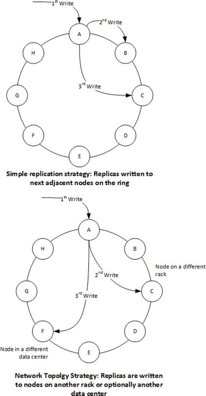
Figure 8-13. Replication strategies in Cassandra
Cassandra uses snitches to help optimize read and write operations. A variety of snitches may be configured.
- The simpleSnitch returns only a list of nodes on the ring. This is sufficient for the simple replication strategy we discussed in the previous section.
- The RackInferringSnitch uses the IP addresses of hosts to infer their rack and data center location. This snitch supports the network aware replication strategy.
- The PropertyFileSnitch uses data in the configuration file rather than IP addresses to determine the data center and rack topology.
In addition, all snitches monitor the read latency for requests and use this to build a statistical model that can route requests to the best-performing nodes.
Specialized snitches exist that understand the networked topology inside various cloud platforms, such as Amazon EC2.
Summary
In this chapter we’ve reviewed distributed database patterns for traditional relational databases and for several nonrelational systems. Relational database architecture was developed in an era of large, monolithic database servers, and most relational databases still run as a single instance. However, shared-nothing clustering is commonplace in massively parallel data warehouses, and Oracle has a commercially successful shared-disk clustered RDBMS.
We looked in detail at three distributed nonrelational database systems. MongoDB uses a combination of sharding and replication to enable distributed processing. HBase leverages the distributed file system of the Hadoop Distributed File System together with a range-partitioning strategy to achieve a highly scalable solution. Cassandra uses the consistent hashing scheme pioneered in Amazon’s Dynamo system to create a symmetrical clustering solution in which no master servers are required.
In a distributed database, multiple copies of data are typically maintained across the cluster. In the next chapter, we’ll see how these databases manage data consistency within such a distributed system.