
![]()
An Interactive Drum Set
In this chapter, we’re going to build an interactive drum set. We’re not going to build the actual drum set, of course, but we’re going to enhance a drum set by placing a few sensors on some of the drums, which will give us input on each drum hit. We’ll use that input to trigger some samples in various ways. We’re also going to use a few foot switches to change between various types of sample playback, but also to activate/deactivate each sensor separately.
The sensors we’re going to use are simple and inexpensive piezo elements, the ones used for contact microphones. We’re going to build four of these in such a way that it’s easy to carry around and set up, so you can use this setup in gigs you’re playing. This time, we’ll use the Arduino Uno since this project is not going to be embedded anywhere, but we’ll be using it with our personal computer. To make our lives easier, we’ll use the Arduino Proto Shield, a board that mounts on top of the Arduino Uno with solder points that give easy access to all Arduino pins.
Parts List
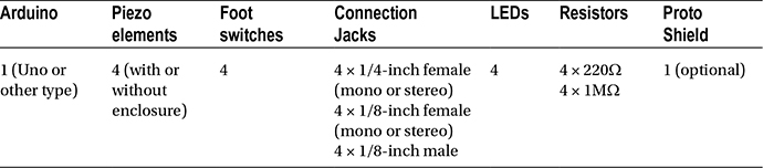
Table 7-1 lists the components that we’ll need to realize this project.
Table 7-1. Parts List
Other Things We’ll Need
In this project, we’ll use an abstraction I’ve made: [guard_points_extended]. You can find it on GitHub at https://github.com/alexdrymonitis/array_abstractions. All the rest will be explained in detail throughout the chapter.
First Approach to Detecting Drum Hits
Piezo elements can be used with the analog pins of the Arduino. They provide voltage that corresponds to the vibration it detects. Our sketch will be based on the Knock tutorial, found on the Arduino web site, but we’re going to change it quite a lot to fit the needs of this project. What we essentially want is to detect drum hits. This can be easily achieved just by reading the analog pins of the Arduino and printing their values over to Pd. Since these sensors can be quite sensitive, we’re going to apply a threshold value, below which nothing will be printed. Listing 7-1 shows a sketch very similar to the Knock tutorial sketch.
This code is rather simple and doesn’t need a lot of explanation (or comments). All we do is set the number of sensors we’re using (which must be wired from analog pin 0 and on, so that the for loop on line 9 will work as expected) and read through their analog pins. If the value of each pin is higher than the threshold value we’ve set on line 1, then we print that value with the tag "drum" followed by the number of the pin. Notice the high baud rate we’re using in line 5. Since we want to detect every single hit on each drum, a high baud rate (the highest the Arduino Uno can handle) is desired here.
First Version of the Circuit
Figure 7-1 shows the circuit for the code in Listing 7-1. You don’t really need to have four piezo elements; you can use as many as you have. Just make sure you set the correct number on line 1 of your code. Also, you can test the circuit in Figure 7-1 on some hard surfaces if you don’t have a drum set available. Using drumsticks or something similar will work better than knocking on these surfaces with your hands.
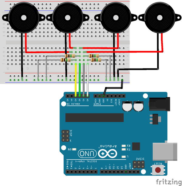
Figure 7-1. Four piezo elements circuit
The piezo elements shown in Figure 7-1 are enclosed in a hard case. Some electronics stores have these kinds of piezo elements, but you can also use the ones without an enclosure. Of course, the enclosure protects the sensor, which might be desired, especially during transportation (you don’t want to find your sensor with its wires broken when you arrive at your gig venue for your setup and sound check). Both types of sensors—with and without the enclosure—come with wires soldered on them, so all you need to do is extend the wires to the length you want. Also, the enclosed sensors are easier to mount, since you can use duct tape straight on them without worrying that untaping them will rip off the wires. Even with the enclosure, these sensors are pretty cheap.
The resistors used in this circuit are 1MΩ resistors, which connect the positive wire of the sensor to ground. Other than that, the circuit is pretty simple and straightforward.
Read the Drum Hits in Pd
Figure 7-2 shows the Pd patch that you’ll need for this circuit and the Arduino code to work with (you probably already guessed how to build this patch anyway).
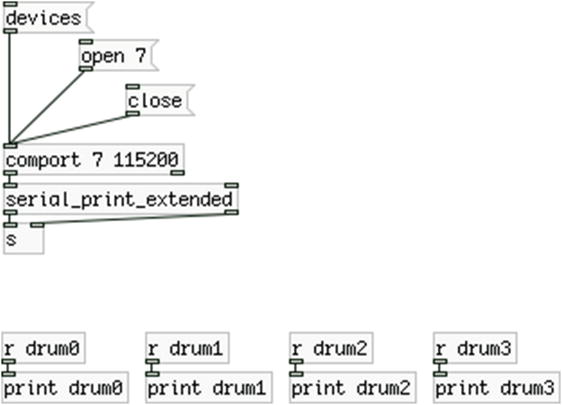
Figure 7-2. Pd patch that works with the Arduino sketch in Listing 7-1
Instead of number atoms, we’re using [print] for each sensor for a reason. Try some hits on each drum (or any hard surface you’re using) with a drumstick. What you’ll probably get is a series of values instead of a single value. This is because the piezo element is an analog sensor, and the values it sends to the Arduino are a stream of numbers representing a continuously changing electrical current. Let’s say that we hit the first drum (or whatever we’re using as a surface) with a drumstick. As the for loop on line 9 goes through the analog pins, it will detect a value greater than the threshold on the first analog pin, and it will print that value. Then it will go through the rest of the pins and start over. When the loop starts over, the surface of the drum we’ve hit will still be vibrating, and pin 0 will still be giving values greater than the threshold, so the loop will again print these values to the serial line. Getting so many values per hit is rather messy, so it’s better if you receive only one value, and preferably the highest value of the hit. We can do that in Pd or Arduino. I’m going to show this both ways. It will then be up to you what you choose.
Getting the Maximum Value in Arduino
To get the maximum value from all the values above the threshold is a rather easy task. All we need to do is check every value above the threshold if it’s greater than the previous one. This is done by calling the max function and checking every new value against the previous one. Listing 7-2 shows the code.
Lines 3 to 5 define three new arrays. The first one, sensor_max_val, will be used to store the maximum value of each sensor, as its name suggests. The other two are used to see if we’ve just crossed the threshold from above to below. The loop function begins the same way it did in Listing 7-1. Again, we’re printing all values above the threshold for comparison with the highest one to make sure that our code works as expected. In line 19, we set the current element of sensor_thresh to 1, denoting that we’re above the threshold. In line 20, we test the value of the sensor to see if it’s greater than the previous one.
We achieve this by comparing the current element of the sensor_max_val array against the value stored by the sensor, calling the max function. This function takes two values and returns the greater of the two. At the beginning, the sensor_max_val array has no values stored, so whatever value is read and stored in the sensor_val variable will be greater that the current element of the sensor_max_val array, so that value will be stored to the current element of the sensor_max_val array.
If the next time the for loop goes through the same sensor, its value is still above the threshold, if the new value is greater than the previous one, again line 20 will store the new value to the corresponding element of the sensor_max_val array, but if it’s smaller, then sensor_max_val will retain its value. Even though we’re assigning to the sensor_max_val array the value returned by the max function, during the test, the sensor_max_val array retains its value. Only if its value is smaller than the value of sensor_val will the sensor_max_val array change, otherwise max will assign to it its own value, since it was the greatest of the two. After we store the maximum value, we update the old_sensor_thresh array according to the corresponding value of the sensor_thresh array. We’ll need these two values when we drop below the threshold.
Updating the sensor_thresh Array
If we drop below the threshold, we set the current element of the sensor_thresh array to 0, and then we test if its value is different from that of the old_sensor_thresh array, in line 25. If it’s the first time we drop below the threshold after a drum hit, this test will be true, since the old_sensor_thresh array won’t have been updated yet and its value will be 1. Then we print the maximum value stored and we set the current element of the sensor_max_val array to 0. If we don’t set that to 0, the next time we hit the drum, the values of the sensor might not go over the last maximum value. And if sensor_max_val has retained its value, the max function in line 20 will fail to store the new maximum value to sensor_max_val, since sensor_max_val is part of the test.
After we’ve checked whether the current element of the sensor_thresh and the old_sensor_thresh arrays are different, we update the old_sensor_thresh array. This way, as long as we don’t hit the drum, the test in line 25 will be false and we’ll prevent the Arduino from printing the same maximum value in every iteration of the for loop.
Reading All Values Above the Threshold Along with the Maximum Value
Figure 7-3 illustrates the Pd patch for the code in Listing 7-3. Upload the code to your Arduino. (You’ll need to send the message “close” to [comport] in Pd if you have the previous patch still open; otherwise, the Arduino’s serial port will be busy and the IDE won’t be able to upload code to the board.) Open its serial port in Pd. Now whenever you hit a drum, you’ll get all the values that were above the threshold printed as drum0, drum1, and so forth, and the highest value of each sensor printed as highest0, highest1, and so on.
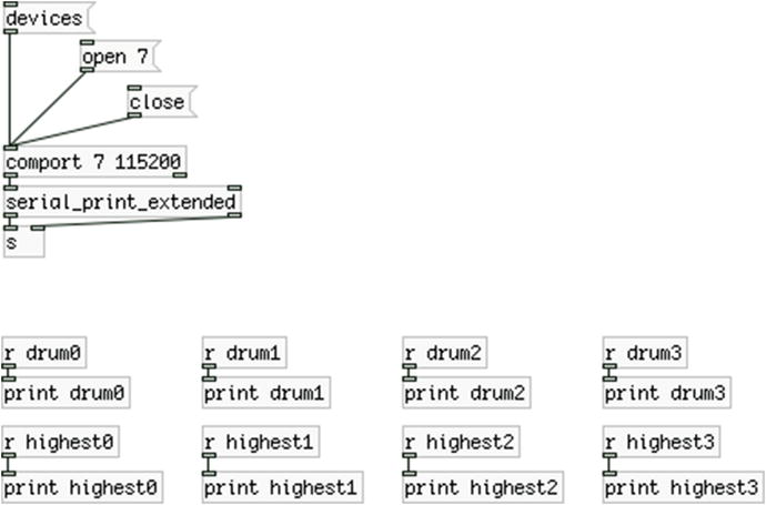
Figure 7-3. Pd patch that works with the code in Listing 7-2, for testing the code and circuit
What you’ll probably notice is that you’ll probably get more than one highest values with a single drum hit. Every time you hit a drum, the sensor values cross the threshold, and the code gives you the highest of the values, but the sensor values might drop below the threshold and then rise above it again, all within the same drum hit. Don’t forget that this is an analog signal that fluctuates as long as the drum surface vibrates. Figure 7-4 illustrates this.
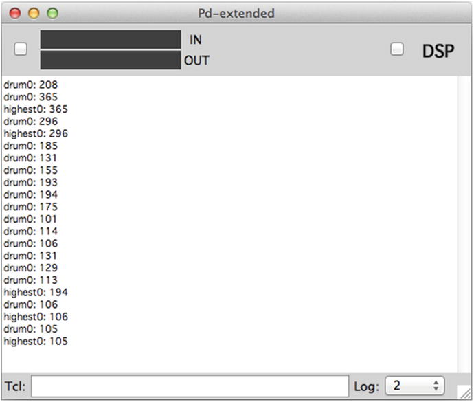
Figure 7-4. Multiple highest values with a single hit
Debouncing the Fluctuation Around the Threshold
This is a bit tricky to overcome. What we need to do is define a debounce time, before which the maximum value won’t be printed to the serial line, but only saved. If the sensor values go above the threshold in a time shorter than the debounce time, then we’ll keep on testing to get the maximum value. Only when the debounce time is over will we print that value to the serial line. Listing 7-3 shows the modified code that solves this problem.
This code is a bit more complex than the code in Listing 7-2, as we need to overcome a pretty complex problem. In the beginning of the code, we define some variables and constants that we might need to change, but these are the only values; the rest of the code remains untouched. Lines 8 to 16 define some arrays for the sensors. All these arrays are necessary to detect whether the values rising above the threshold are within the same drum hit, or whether it’s a new drum hit.
In the loop function, the lines 23 to 29 are identical to the beginning of the loop function in Listing 7-2. In line 27, we check whether we’ve risen above the threshold for the first time, by doing the reverse test we did in Listing 7-2, when we went below the threshold. If it’s true, we increment the value of the corresponding element of the sensor_above_thresh array, which counts how many times we’re going above the threshold when coming from below it. Then we go on and retrieve the maximum value of the sensor, like we did in Listing 7-2.
In line 34, the code of else starts. At the beginning, we set the current element of the sensor_thresh array to 0, like in Listing 7-2 and what we do then is take a time stamp of when the current sensor was measured to be below the threshold. We do that by calling the function millis(). This function returns the number of milliseconds since the program started (since we powered up the Arduino, or since we’ve uploaded the code to it). This function returns an unsigned long data type, but the sensor_below_const array is of the type int. To convert the data type that the millis function returns, we cast its returned value to an int, by calling it like this:
(int)millis();
This way the value millis returns will be converted to an int. It’s probably OK not to do this casting at all, and call millis as if it returned an int, but casting its value is probably a better programming practice, and it’s also safer.
Mind that the time stamp is not about when the sensor values drop from above the threshold to below it, but whenever the sensor is measured to be below the threshold, which will happen in every iteration of the for loop, if the sensor is below the threshold (meaning, for as long as the corresponding drum is not being hit).
In line 38, we’re checking if the sensor values have dropped from above the threshold to below it. If it’s true, we’re taking a new time stamp, this time denoting the moment we dropped below the threshold. We’re going to need these two time stamps for later. After taking the new time stamp, we update the old_sensor_thresh array.
In line 43, is where we’re checking whether we have just dropped below the threshold (which means that we might go up again, and we don’t want to print any values), or if we have passed the debounce time, so we need to print the maximum value to the serial line. We’re checking if the difference between the two time stamps is greater than the debounce time we’ve set in line 5, which is 10 (milliseconds). Since this test will be made every time a sensor is measured below the threshold, which will happen for as long as a drum is not being hit, we need to take care that the code in this test is not being executed every single time, but only after a drum hit. This is where the sensor_above_thresh array is helpful. In line 45, we’re checking whether the current sensor counter in the sensor_above_thresh array is above 0. If it is, it means that the sensor has gone above the threshold at least once, so there is some data we should print to the serial line. If the test of line 45 is true, we’re printing the maximum value of all the values of the sensor, including those that went from below the threshold to above it, within the debounce time. After we print the value, we set to 0 the elements of the sensor_max_val and sensor_above_thresh arrays, so we can start from the beginning when a new drum hit occurs.
We have added only a few things to the code in Listing 7-2 and we have overcome the problem of multiple highest values with a single drum hit. All we needed was two time stamps and a debounce time. You can use the same Pd patch (the one in Figure 7-3) with this code. Compare the results with the code in Listing 7-2 and the one in Listing 7-3. You’ll see that with the latter you get only one “highest” value per hit, whereas with the former you might get more. If you still get more than one “highest” value with the code in Listing 7-3, try to raise the debounce time in line 5. Of course, we don’t need the raw “drum” values; they’re there only for testing. Experiment with the debounce time, try to set it to the lowest possible value, where you don’t get multiple “highest” values with one hit, so that your system is as responsive as possible. Another thing to change can be the threshold value, which will determine how responsive to your playing the system will be. We’ll leave that for later, as it’s better if we control this from Pd instead of having to upload new code every time.
Getting the Maximum Value in Pd
Now let’s see how we can achieve the same thing in Pd. We’ll collect all the values printed by the Arduino, and when we’re sure we’re done with a drum hit, we’ll get the maximum of these values. We’ll take it straight from the second step, where we define a debounce time, so that we don’t get multiple maximum values for one drum hit. Even though we’re checking for the maximum value in Pd, we still have to start with the Arduino code. Listing 7-4 shows the code.
This code is very similar to the code in Listing 7-3. What we don’t do here is check the maximum of the values that are above the threshold since we’ll do it in Pd, we only print them to the serial line. Again, we’re taking the same time stamps and we’re checking if we’ve crossed the debounce time so we can get the maximum value in Pd. If we’ve crossed the debounce time, we send a bang to Pd under the same tag, "drum" followed by the number of the sensor. This bang will force the maximum value to be output. Figure 7-5 shows the Pd patch for this code.
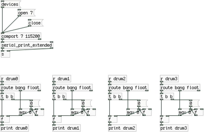
Figure 7-5. Pd patch that calculates the maximum value of each sensor
This patch is slightly more complex than the patch in Figure 7-3. Since both the values of the sensor, but also the bang are printed to the serial line under the same tag, we’ll receive them with the same [receive]. We use [route bang float] to distinguish between floats (remember, in Pd all values are floats, so even though we’re printing integers from the Arduino, Pd receives them as floats), and bangs. Each float goes to a [max 0], which outputs the maximum value between its arguments and the value coming in its left inlet to two [f ]s. [max]’s output goes to the left (hot) inlet of the [f ] on the right side, which will immediately output that same value and send it to the right (cold) inlet of [max]. This way the argument of [max] will be overridden by the output of the right [f ], which is essentially the output of [max] itself. The same output goes to the right inlet of the [f ] to the left side. This way, we store the maximum of all incoming values. It is the same as the following line of code in Arduino:
sensor_max_val[i] = max(sensor_max_val[i], sensor_val);
When we receive a bang, we first set 0 to [max], so we reset its initial argument for the next drum hit, and then we bang the left [f ] to force it to output its value. To test whether this works as expected, connect a [print raw0] (type the number of each sensor, such as raw1, raw2, and so forth) to the middle outlet of [route], which outputs all the incoming floats, and see if the value printed as drum0, drum1, and so on, is equal to the maximum value of all the values printed as raw0, raw1, and so forth in Pd’s console.
Mind that we don’t use [trigger] to send the output of [max] to the two [f ]s, but instead we use the fan out technique. The order these values are being output depends on the order the objects were connected, and there’s no way to really tell how these objects were connected (only by looking at the patch as text, but this is not something very helpful anyway, plus its rather confusing). In this case, the fan out doesn’t affect the patch at all, since there’s no other calculation made depending on the order of this output. In general, it’s better to use [trigger], but in such cases (like this or the case of a counter), it’s OK to use fan out.
Again, you might want to experiment with the debounce time set in the Arduino code to make your system as responsive as possible. Make sure that you get only one value printed as drum0, drum1, and so forth for every drum hit. If you start having more than one, then you should raise the debounce time a bit. Test this until you get the lowest debounce time possible.
What we’ve done here is take away some complexity from the Arduino code and add it to the Pd patch. This shows us that the same thing is possible in different programming languages (well, they’re not so different, Arduino is written in C++ and Pd in C). Now let’s start building on top of this to make our project more interesting.
Having Some Fun Before We Finalize
This project is aimed at playing various samples stored in arrays in the Pd patch, every time we hit a drum. There are various ways to play back a sample. Before we build the circuit and code of the Arduino, let’s first have some samples play back in reverse every time we hit a drum.
I have downloaded some drum samples from freesound.org. Since it’s a drum set, it could be nice to have a drum sound corresponding to each kind of drum (kick drum, snare drum, and so forth), playing backward every time we hit it. Figure 7-6 illustrates the Pd patch.
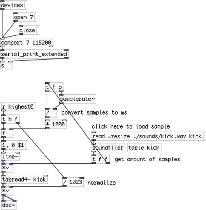
Figure 7-6. Pd patch playing a kick drum sample backward on each drum hit
I’ve used the code in Listing 7-3 instead in Listing7-4, where the maximum value is being calculated in the Arduino code and not Pd, just to make the patch a bit simpler. If you want to calculate the maximum value in Pd, replace [r highest0] in Figure 7-6 with the part of the patch in Figure 7-5 that calculates the maximum value ([r highest] should be replaced by [r drum0], and [print drum0] should not be included). Of course, now we don’t need to print the raw values that are printed with the "drum" tag, and we’re going to change that as we develop the Arduino code even more. For now, we use the code in Listing 7-3 as is to make some sounds with Pd.
The first thing you need to do is click the “read -resize ./sounds/kick.wav kick” message, which will write the sample called kick.wav to the kick table. This sample is in a directory (folder) inside the directory of the patch, hence the path ./sounds/kick.wav. We could also use [openpanel] instead which would open a dialog window with which we could navigate to the sample, but if we know the location of the sample, it’s easier if we load it this way, since we can also automate it with a [loadbang].
Once we click the message, the kick.wav file will go through [soundfiler], which will first load the sound file to the specified table and will output the number of samples of the sound file. This number goes to two locations: [t f b] on the right side of the patch and [*~ ]. We’re reading the sound file with [line~], which makes a ramp from 1 to 0 (we’ll read the sound file backward). To read the whole sound file we need to multiply this ramp by the number of samples of the file, so instead of going from 1 to 0, it will go from the total length of the sound file to 0. We could have used this value to set the ramp of [line~] instead of sending it the message “1, 0 $1”; but further on, we’ll use different ways to read sound files, so it’s better if we have a generic ramp and multiply accordingly.
The part where the number of samples of the sound file goes to [t f b] calculates the length of the sound file in milliseconds. This is a pretty straightforward equation. We divide the amount of samples by the sampling rate (using [samplerate~]), which yields the length of the sound file in seconds, and we multiply by 1000 to convert it to milliseconds. We store that value in [f ], which waits for input from the Arduino. As soon as we hit the drum with the first sensor on, [r highest0] will output the maximum value of the sensor. This value goes first to [/ 1023], since 1023 is the maximum value we can get from the Arduino to be normalized to 1, and set the amplitude of the sound file, and then it bangs [f ] which goes into the message “1, 0 $1”. This message means to “go from 1 to 0 in $1 milliseconds,” where $1 will take its value from [f ], which is the length of the sound file in milliseconds. As soon as you hit the drum, you should hear the sample playing backward, with its loudness corresponding to how hard you hit the drum. This can be a nice echo-like effect.
Working Further with the Circuit and Arduino Code
Before we go on and see other ways we can play back the various audio files, let’s work a bit more on the circuit. Since we’re going to have a few different ways to play back sounds, we must have a convenient way to choose between these playback types. Since this is an interactive drum set, the hands of the performer might be available, but it’s still not easy to navigate to a certain point on a laptop screen with the mouse while performing. It’s better if the performer has an easy-to-use interface, which he/she can control at any time. A good interface is one with quite a big surface, which is easy to locate. For this project, we’re going to use foot switches. These switches will control the playback type of the sound files, but also whether a sensor is active or not. Like the project in Chapter 6, since we have an interface to control some aspects, why not have the ability to control the activity of the sensors, since this gives the performer the freedom to choose whether to play with or without the sensors at any given moment.
We’re going to enclose the circuit in a box so that it’s easy to carry around, since you may want to take it with you at some gig. We’ll also use LEDs to indicate the activity of each sensor, so that you know which sensors are active and which are not, at any given moment. Before we build the circuit on a perforated board and put it in a box, we must build it on a breadboard and test if it works as expected.
Adding Switches and LEDs to the Circuit and Code
Since we have four sensors in our circuit, we’re going to use four foot switches to control them. This applies some limitation to how many different kinds of playback we’ll have, but when building interfaces we must set strict priorities, which concern functionality, flexibility, ease of use and transport, among others. The more control we want over a certain interface, the more the circuit will grow, and this can lead to rather complex circuits, which may not be desirable. If you want to add more foot switches or piezo elements to your project, you’re free to do it. This chapter focuses on four of each.
To test the circuit and code we’ll first use tactile switches (breadboard-friendly push buttons). Once it’s all functioning properly, we’ll go on and enclose the circuit in a box, using foot switches. Figure 7-7 shows the circuit with four push buttons and four LEDs.
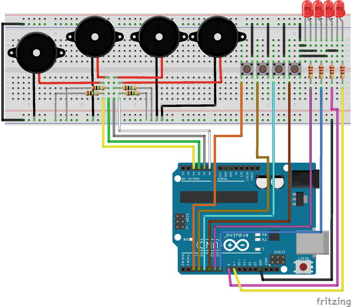
Figure 7-7. Full test circuit
There’s nothing really to explain about the circuit. We’ll use the Arduino’s integrated pull-up resistors for the switches, and we’re using 220Ω resistors for the LEDs, and 1MΩ resistors for the piezo elements. What I need to explain is the code that will work with this circuit. First, let’s try to make the switches control the activity of the piezo elements. The code is shown in Listing 7-5.
The additions are very few, we’ve only added two arrays sensor_activity, and all_switch_vals. The first determines whether each sensor is active or not , as its name suggests. Since we only need this array to determine whether a state is true or false, we define it as a bool. The second array is used to test whether a switch has changed its state, otherwise the code of the for loop of line 31 would be executed constantly.
In the setup function, we set values for the two arrays and the mode for the digital pins. We also set the state of the LEDs according to the values of the sensor_activity array. By default, all sensors are active, so all the LEDs will turn on as soon as the Arduino is powered.
In the loop function, we run through all the switches and test if their state has changed (whether they are being pressed or released). If it has, we’ll check if the switch is pressed in line 35, and if it is, we’ll switch the corresponding value of the sensor_activity array and update the state of the corresponding LED. Then in line 39, we update the corresponding value of the all_switch_vals array so that the test in line 34 will work properly when the for loop goes through the same switch pin again. This update happens only if a switch is pressed, so in line 42, we update the all_switch_vals array, in case the state of a switch has changed, but we’re releasing it.
Then in line 46, we go through the sensor pins, and in line 47, we check the activity of each sensor. If the sensor we’re at is active, then the code that reads its values, gets the maximum, and prints it is executed. If the sensor is not active, then we go on to the next sensor. The code inside the if of line 47 is the same as with Listing 7-3, only this time we’re not printing every value that’s above the threshold, but only the maximum of all the values with the "drum" tag instead of "highest". Figure 7-8 illustrates the Pd patch for this code. It’s essentially the same as with Figure 7-3, only there are not [r highest] objects, since we’re not printing any values with this tag.
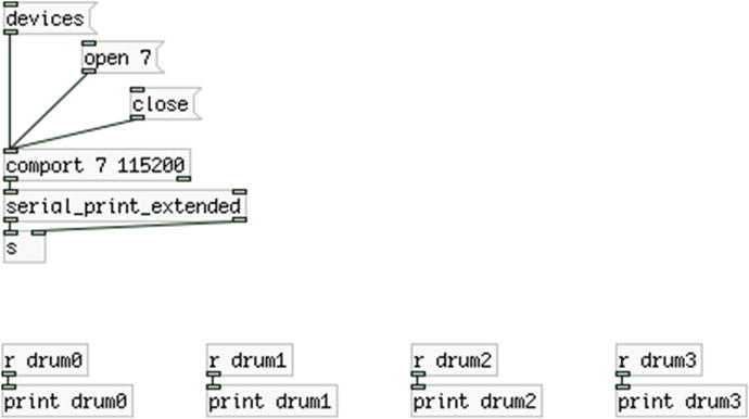
Figure 7-8. Pd patch for the Arduino code in Listing 7-5
With this code and patch, you have control over to which sensor is active and which is not, having direct visual feedback from the corresponding LEDs. Try to deactivate a sensor and hit its drum. Check the Pd console to see if you get any values printed, you should not. This gives us great flexibility, as we might not want to trigger samples all the time, but at certain moments during our playing.
Using the Switches to Control Either Playback Type or Sensor Activity
Now to the next step, where we’ll use the switches to control two things, playback type or sensor activity. To do this we’ll use the first switch to determine which of the two aspects we’ll control. We’ll do this by checking for how long we keep the switch pressed. If we keep it pressed for more than one second, we’ll switch the type of control. If we keep it pressed for less than one second, the switch will control whatever the other switches control. (If the control type is set to sensor activity, it will control the activity of the first sensor; otherwise, it will control the type of playback.)
To do this, we again need to take time stamps of when we press and when we release the first foot switch. We’ll then compare the difference between the two time stamps; if it’s more than 1000 (milliseconds), we’ll switch the type of control the switches will have. I’m not going to show all the code because the greatest part of it is the same as before. I’ll only show the additions we need to make. Listing 7-6 shows some new variables and arrays we need to create. Of course, all these strings should be written in one line in the Arduino IDE, they just don’t fit in one line in a book.
The first array all_switch_vals, was there in Listing 7-5 as well, but we’re including it here because these variables and arrays all concern the switches. The second variable is an int that sets the type of control. You’ll see how this is done in Listing 7-7. Lines 4 and 5 define a new type that we haven’t seen before: String. String is a built-in class in the Arduino language, which manipulates strings, therefore its name. This class enables us to easily create string objects, even arrays of strings. Line 4 defines the strings "playback" and "activity", which we’ll use in Pd to label the type of control the foot switch currently has. Line 5 defines four strings that have to do with the type of playback we’ll use. "ascending" means that we’ll play a sound file a few times repeatedly, where each time it will be played faster and at a higher pitch. "descending" means the opposite. "backwards" means just that, and "repeatedly" means that we’ll play a short fragment of the sound file many times repeatedly, creating a sort of tone. We’ll see all these types of playback in practice when we build the Pd patch. Place this chunk of code at line 15 in Listing 7-5, where we set the all_switch_vals array.
Listing 7-7 shows the for loop for the switches. This must replace the code in Listing 7-5 from line 31 to line 44. Mind that if you have added the code in Listing 7-6, these line numbers will have changed.
This is quite more complex than the for loop for the switches in Listing 7-5. The first thing we do after we read each digital pin is check whether its state has changed, which is the same as in Listing 7-5. Then in line 5, we’re checking if the switch that is being changed is the first one, by using the variable i with the exclamation mark. If it’s the first one, i will hold 0, and the exclamation mark will make it 1, which is the same as true. If i holds any other value (1, 2, or 3), the exclamation mark will make it 0, which is the same as false. In line 6, we define two local variables for the two time stamps we need to take, which are both static, so even though they’re local, even when the function in which they’re defined is over, they will retain their values.
In line 7, we check if the first foot switch is being pressed, and if it is, we take a time stamp of when we pressed it, and then update all_switch_vals so testing if the switch’s state has changed will work properly. else in line 11 will be activated if the first switch is being released, where we’re taking another time stamp of when that happened, and we again update all_switch_vals. Then in line 14, we’re testing the time difference between the two time stamps. If it’s greater than 1000 we switch the value of the control variable, and we print the corresponding string from the control_type string array, where if control is 0, we’ll print "playback", and if it’s 1, we’ll print "activity". By default, control is 1, so the first time we’ll hold the first switch pressed for more than a second, the control type will change to "playback".
If the difference between the two time stamps is less than 1000, we first check the type of control the switches have. If it’s 1, releasing the foot switch will switch the state of the first element of the sensor_activity array, and this value will be written to the pin of the first LED. If control is 0, we’ll print the first element of the playback_type string array, which is "ascending".
Afterward, we’re updating the all_switch_vals array right before else of line 11 has ended, which is called if the first switch is being released. It’s very important to place the updates of the all_switch_vals array in the right places, otherwise the code won’t work properly. In this code, we’re separating the first foot switch from the rest, plus we’re separating what happens when we press the switch from what happens when we release it. For the rest of the switches we only care about releasing the switch. So we need to update the all_switch_vals array every time we press or release the first switch and every time the state of any of the other switches changes. That’s why this array is being updated in one more place in line 45.
In line 32, we have an else that will be executed if a state change has been detected, but it was not the first switch. In line 33, we’re checking if the switch is being released. In Listing 7-5, we were checking when a switch was being pressed. Since for the first switch we can’t determine what we want to do when we press it, but only when we release it, because we’re counting the amount of time we held the switch pressed, it’s better to use the release for the rest of the switches, for the compatibility of the interface. Depending on the type of control the switches have, we’ll switch the current element of the sensor_activity array and write that value to the corresponding LED, or we’ll print the corresponding element of the playback_type string array, which will be "descending", "backwards", or "repeatedly". After updating the all_switch_vals array, the loop ends and we go on to read the pins of the sensor. This is not included in Listing 7-7 because, as I already mentioned, it is exactly the same in Listing 7-5.
Building the Final Pd Patch
We’re now at a point where we can start building the actual patch for this project. This patch will consist of three different levels, the audio file playback, the Arduino input, and the main patch. We’ll first build the patch that reads the audio files, and then the patch that receives data from the Arduino and triggers the playback. Then we’ll go on and put everything together in the main patch for this project.
Building the Audio File Abstraction
Since the only difference between each audio file playback for each sensor will be the table where we’ll load the audio file to, it’s better if we first make an abstraction that we can duplicate for each sensor. We can set the name of the table via an argument, along with some other data that we’d like to pass, but different for each abstraction. This abstraction should take a bang and play back the audio file loaded on the table specified via an argument, in a way set by the switches. Figure 7-9 illustrates this abstraction.
The heart of this abstraction is [line~], which is the index for the table of the sound file, but also for the window that smooths out the beginning and the end of the file. [loadbang] goes first to [del 100], because in the parent patch we first want to load the audio files to the tables and then do any calculations depending on those files, so we give some short time to Pd when the patch loads to first load these files to the tables. After this 100 milliseconds delay, we get the size of the table each abstraction reads with [arraysize $1]. $1 will be replaced by the first argument of the abstraction, which will be the name of the table with the audio file we want to read. The value output by [arraysize] is the number of samples of the audio file, since the table where it will be loaded will be resized to a size that will fit all the samples of the file. This value goes to two locations, first it goes to [*~ ] next to which there is the comment “this is the total length of the table”. We’ll set [line~] to go from 0 to 1, so we’ll need to multiply it by the number of samples of the audio file so that [tabread4~] can output the whole file.
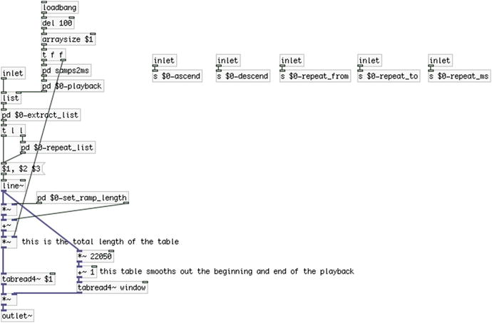
Figure 7-9. The read_sample abstraction
Converting Samples to Milliseconds and Dealing with the Sampling Rate
The second location the size of the table goes is the [pd samps2ms] subpatch, which calculates the amount of milliseconds it will take to read the whole audio file. This is very often useful; you might want to consider making an abstraction so that you can use it frequently. The contents of the subpatch are shown in Figure 7-10. The calculations in this subpatch are pretty simple, so I won’t explain it. One thing that I need to mention at this point is that you should take care of the sampling rate your audio files have been recorded in. If you download sounds from freesound.org, the sampling rate of each sound is mentioned on the sound’s web page. Otherwise, you can get this information from your computer, if you have stored sound files in your hard drive. All the audio files that you load in your patch should have the same sampling rate. Pd must run at the same sampling rate too for the audio files to be played back properly. To change Pd’s sampling rate, go to Media ![]() Audio Settings….
Audio Settings….
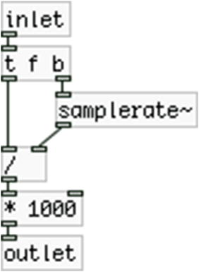
Figure 7-10. Contents of the samps2ms subpatch
Creating Different Types of Playback
After [pd samps2ms] has calculated the amount of milliseconds an audio file takes to be read, it sends its value to [pd $0-playback], the contents of which are shown in Figure 7-11. In this subpatch, we’re creating lists according to the string that sets the type of playback, sent by the Arduino. The only straightforward playback type is “backward” which outputs the list “1 0 $1”, where $1 is replaced by the milliseconds it takes to read the audio file. This list will be sent to [line~] which will make a ramp from 1 to 0, lasting as long as it needs to read the audio file at normal speed, which will cause [tabread4~] to read the audio file backward.
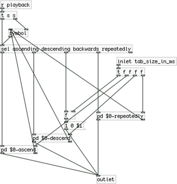
Figure 7-11. Contents of the $0-playback subpatch
The rest of the playback types are inside subpatches because their calculations are not so simple, and putting them in subpatches makes the patch a bit tidier. They are illustrated in Figures 7-12 through 7-15.
In the “ascend” subpatch we receive, store, and output the audio file length in milliseconds in [f ], and we run a loop for as many times set by the second argument to the abstraction, which is stored in [$2 ]. We need to store the value in case we want to set a different number of repetitions for this playback type with a value entered in the second [inlet] of the abstraction. By sending the milliseconds length in the left inlet of [f ], we both output it and save it at the same time, so we can use it again even if [inlet tab_size_in_ms] doesn’t output a new value.
[until] will bang [f ] below it as many times the loop runs. At the beginning, [f ] holds the length of the audio file in milliseconds, and every time it is banged, it outputs it and it also gets divided by 2, so it stores half that value. This values goes to the message “0 1 $1”, which is the list that will be sent to [line~] to make a ramp from 0 to 1 in the time specified by $1. (Remember that $1 in a message means the first value of a list—in this case, it’s just one value list—that arrives in the inlet of the message. $1 in an object contained in an abstraction means the first argument given to the abstraction. The interpretation of $1—or $2, $3, and so forth—is totally different between messages and objects). The list of this message goes to [list prepend] which outputs the lists it gets in its left inlet to [t l l] ([trigger list list]). [t l l] will first send the list to the right inlet of [list prepend], and the latter will store that list, and then it will send it to the right inlet of [list] at the bottom, which will also store it.
This way we can create a growing list, since [list prepend] will prepend anything stored in its right inlet to anything that arrives in its left inlet. So, if the length of the audio file is 1000 milliseconds, the message that goes to [list prepend] will first output “0 1 1000”. [list prepend] will output this list and it will also store it in its right inlet. The second time, the message will send “0 1 500”, which will go to the left inlet of [list prepend] and the previous list will be prepended to it, resulting in [list prepend] storing the list “0 1 1000 0 1 500”. The third time the message will output “0 1 250”, so the list stored in [list prepend] will be “0 1 1000 0 1 500 0 1 250”, and so on. This will go on for as many times as we’ll set via the second argument to the abstraction. All these lists will go to the right inlet of [list] at the bottom of the subpatch, and every time [list] will replace whatever it had previously stored with the new list that arrives in its right inlet. When [r playback] in the subpatch in Figure 7-11 receives the “ascending” symbol, it will bang [pd ascend] which will output the final list stored in [list], which will be a set of lists of three elements, 0, 1, and the decreasing time in milliseconds. This full list will go to the right inlet of [list] in the top-left part of the parent patch of the abstraction, shown in Figure 7-9, which will be banged whenever the corresponding sensor will output a value. We’ll see later on how this works.
Notice that in Figure 7-12 there’s a [r $0-ascend] which receives values from [s $0-ascend] from the parent patch of the abstraction (Figure 7-9). If we want to change the number of repetitions of the ascending playback on the fly, we can send a value to the second inlet of the abstraction and it will arrive in [pd $0-ascend]. When we receive this value we’ll first bang the right inlet of [list prepend]. This will cause the object to clear any stored list. Afterward, we’ll store the value in [$2 ], so its value will be replaced. Then we’ll bang [f ], which holds the duration of the audio file in milliseconds. And finally we’ll send a bang to the outlet of the subpatch, which will go to [pd $0-playback] (Figure 7-11). This bang is sent to the left inlet of [symbol], which has stored the symbol arriving from the Arduino (“ascending”, “descending”, “backwards”, or “repeatedly”). We do that so we can output the list generated by the subpatch, which is stored in [list] at the bottom of [pd $0-ascend]. If we don’t bang it, [list] won’t output its list and we won’t be able to hear the new setting we made by sending a value in the inlet of the abstraction.
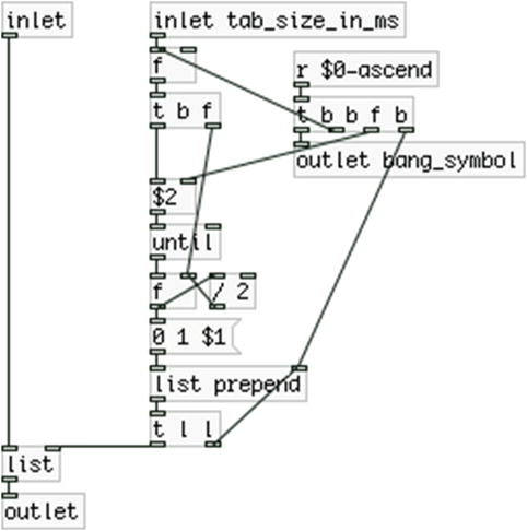
Figure 7-12. Contents of the $0-ascend subpatch
The next one is [pd $0-descend], shown in Figure 7-13. This is very similar to [pd $0-ascend]. Instead of playing the audio file twice as fast (and at a higher pitch) every time, we start by playing it fast, and every time we play it twice as slow, end it at the normal speed (starting at a high pitch and ending at the normal pitch). In this subpatch, we calculate the shortest duration according to the length of the audio file and the number of repetitions, which is set via the third argument, and then we run a loop starting with this shortest duration and every time we double it. Apart from that the rest of the patch works the same way as [pd $0-ascend].
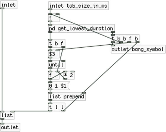
Figure 7-13. Contents of the $0-descend subpatch
I need to explain how the get_lowest_duration subpatch works, which is shown in Figure 7-14. This subpatch runs a loop similar to that of [pd $0-ascend]. We start with the normal duration of the audio file and every time we divide it by two. When we’ve gone through all the iterations of the loop, [sel $3] will bang the final value, which is stored in [f ] at the bottom of the subpatch. This value will then go in [pd $0-descend] and another loop will run, now starting with the shortest duration, every time multiplying by two, ending at the normal duration. Again, we have a long list stored in [list], which we bang whenever we send the symbol “descending” from the Arduino. Notice that [r $0-descend] is in [pd get_lowest_duration], as if we changed the number of repetitions. We’ll need that number in there too to calculate the shortest duration for the audio file. Mind the order of sending that value or a bang and try to understand why we need things to go in this order, so that everything works as expected.
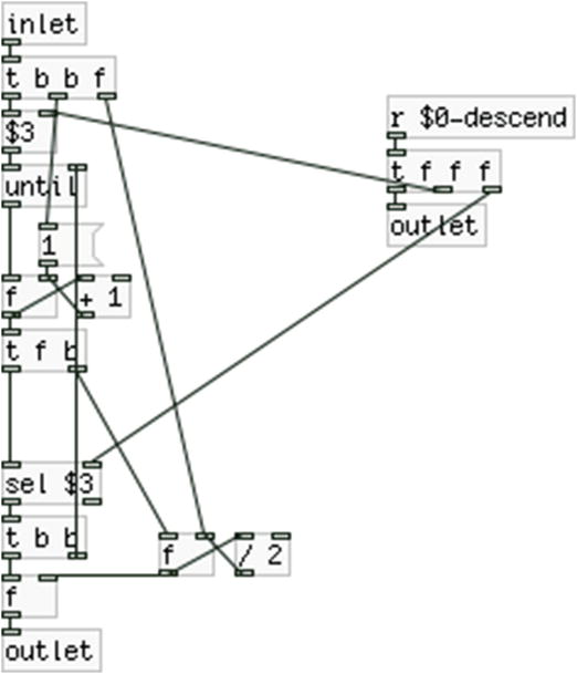
Figure 7-14. Contents of the get_lowest_duration subpatch
Then we go to [pd $0-repeatedly], which is shown in Figure 7-15. This is quite different than the other two subpatches that I’ve explained. In this subpatch, we’re using the fourth and fifth arguments of the abstraction, which are the points of the audio file where we want our repeated playback to start and end. We don’t need to know the length of the audio file, either in milliseconds or samples, to set these two arguments. They are set in some kind of percentage, from 0 to 1, where 0 will be the beginning of the file and 1 its end. What we do in [pd $0-repeatedly] is subtract $4 from $5 to get the duration of the file we want to play back, in a 0 to 1 scale, and then we multiply the result by the length of the audio file in milliseconds. This will tell [line~] to go from 0 to 1 in the time it takes to play the portion of the file we want. In [pd $0-repeatedly] we can see a [s $0-repeat_length] with a comment stating, “goes into [pd set_ramp_length]”. This value (the difference between $4 and $5) will set the amount of scaling and an offset to the ramp of [line~]. If [line~] went from 0 to 1 in the time it takes to read only a portion of the file, which is set via $4 and $5, the result would be that [tabread4~] would read the whole file much faster that its normal speed. Since we’re using the ramp of [line~] to control a smoothing window, in the parent patch of the abstraction, we’re telling [line~] to go from 0 to 1, so that the smoothing window will be read properly, and then we scale its ramp and we give it an offset before if goes to [tabread4~]. All this might start to get a bit complex, but if you go back and forth from subpatch to parent patch, and try to keep track of what’s going on, you’ll understand how things work in this patch. In [pd $0-repeatedly] we have two [receive]s, a [r $0-repeat_from] and a [r $0-repeat_to], which take values from the fourth and fifth inlet of the abstraction. If we want a different portion of the audio file, we can change the values with these two inlets, and the necessary calculations will be done. Again, we store the resulting list to [list], which we’ll bang if the Arduino sends the symbol “repeatedly”. And that’s all about [pd $0-playback], now back to the parent patch.
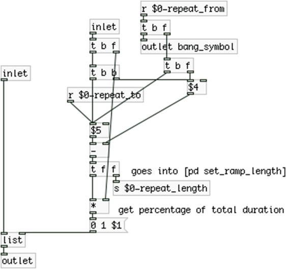
Figure 7-15. Contents of the $0-repeatedly subpatch
In the parent patch we see another subpatch, [pd $0-extract_list], which is shown in Figure 7-16. This subpatch takes input from [list] at the top-left part of the parent patch, which holds the list of the type of playback we want. If we’ve set the playback type to “ascending” or “descending”, then the corresponding subpatches will output a long list, which should be split to groups of three, the beginning of the ramp of [line~], the end of the ramp, and the duration of the ramp. In [pd $0-extract_list] we do exactly that. [list split 3] splits the incoming list at the point specified by its argument. So this object will output the first three elements of its list out its left outlet, and the rest will come out the middle outlet.
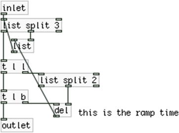
Figure 7-16. Contents of the $0-extract_list subpatch
Since Pd has the right-to-left execution order, [list split] will first give output from the middle outlet and then from the left one. The middle outlet receives the remaining of the list and stores it in [list]. The left outlet outputs the three element list to [t l l], which first outputs this list to [list split 2]. [list split 2] will output a list with the first two elements of the list it received out its left outlet, and the remaining third element out its middle outlet, which goes to the right inlet of [del]. This last value stored in [del] is the ramp time of the first three elements, in milliseconds. After the ramp time has been stored in [del], [t l l] will output the three element list out its left outlet, which goes to [outlet]. From there, it will go to the message “$1, $2 $3” in the parent patch, which tells [line~]: “Jump to the first value of the list, and then make a ramp to the second value which will last as many milliseconds as the third value.” So [line~] will make a ramp from 0 to 1 that will last as many milliseconds as the audio file lasts.
At the same time [t l l] outputs the list through [outlet] in [pd $0-extract_list], it also bangs [del] (actually it first bangs [del] since [t l b] will first send a bang out its right outlet). When [del] receives a bang, it will delay it for as many milliseconds as the value it has stored in its right inlet, which is the amount of milliseconds the ramp takes. So as soon as [line~] finishes with its ramp, [del] will bang [list], which has stored the remaining list, and it will send it to [list split 3], and the whole procedure will start over, every time taking the first three elements of the list, until the list is finished. This way we can have repeated ramps, each lasting half the time of the previous one, in case we’re playback in the “ascending” type, or twice as long, in case we’re playing back in the “descending” type. If we playback in the “backwards” or “repeatedly” type, [pd $0-extract_list] will output one list only, since these two types produce a list of three elements only.
The output of [pd $0-extract_list] goes to [t l l] in the parent patch, which outputs the incoming lists first to [pd $0-repeat_list] and then to the message sent to [line~]. [pd $0-repeat_list] is activated only if we receive the symbol “repeatedly” from the Arduino. What it does is take the list generated by [pd $0-repeatedly] and repeat it for an amount of time set in milliseconds by the sixth argument to the abstraction. It is shown in Figure 7-17. If the Arduino sends the symbol “repeatedly”, we’ll receive it in Pd via [r playback] and [sel repeatedly] will send a bang out its left outlet, which will send 1 to the two [spigot]s. As soon as this subpatch receives a list, it first bangs [del $6], which will have its delay time set via the sixth argument. Then, it will bang [f ] containing 1. Then, it will send the list to [list split 2], which will output the ramp time of the list out its middle outlet into [pipe 0 0 0 0]’s rightmost inlet, and then the same list to the leftmost inlet of [pipe].
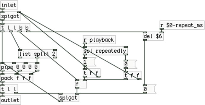
Figure 7-17. Contents of the $0-repeat_list subpatch
[pipe] is like [del], only instead of outputting bangs delayed by a specified time, it outputs numeric values entered in its inlets. It can delay whole lists, where the arguments initialize the lists’ values, and the very last argument is the delay time. Its inlets correspond to its arguments, so sending a value to the rightmost inlet will set a new delay time; sending a list in the leftmost inlet will replace as many arguments as the elements of the list with these elements. If [pd $0-repeatedly] generates the list “0 1 50”, [list spit 2] will send “50” to the rightmost inlet of [pipe], which will be the delay time, and in the leftmost inlet, [pipe] will receive the whole list, which it will delay for 50 milliseconds.
This list goes out three different outlets ([pipe] creates one outlet for each element of the list, the delay time is not included), which are [pack]ed to be sent as a list to [line~]. Since the [spigot]s are open, [t l l] will first send the list back to [pipe], which will again be delayed for 50 milliseconds, and this will go on until [del $6] bangs the message “0”, which will close the lower [spigot]. This way we can send the same list over and over for an amount of time that we specify either via an argument or through the sixth inlet of the abstraction (which goes to [s $0-repeat_ms], received by [r $0-repeat_ms] in [pd $0-repeat_list]). As soon as we send a symbol other than “repeatedly” from the Arduino, the top [spigot] in [pd $0-repeat_list] will close, and incoming lists won’t go through anymore. And this covers how the four different ways of playback are achieved.
The $0-set_ramp_length Subpatch
There’s one more subpatch that I need to explain and we’re done with the [read_samp] abstraction, which is [pd $0-set_ramp_length], shown in Figure 7-18. If you see Figure 7-9 you’ll see that the output of [line~] goes to two destinations, [*~ ] and [*~ 22050]. The first multiplication object ends up in [tabread4~ $1], which reads the audio file stored in the table the name of which is set via the first argument to the abstraction. [*~ 22050] ends up in [tabread4~ window] which reads a smoothing window function which we’ll place in the parent patch of our project. This window will smooth out the beginning and end of each audio file since it may not begin or end smoothly and cause clicks, or in the case of playing back the sound repeatedly, since we won’t be reading the file from beginning to end, even if it’s smooth at its edges, we’ll get clicks for sure. You’ll see this window further on. The point here is that we need the same ramp to control two different things, that’s why we always set it to go from 0 to 1, or the other way around (the smoothing window can be read backward too), and we then scale accordingly, and if necessary, give it an offset too. In [pd $0-set_ramp_length], if we receive the symbol “repeatedly”, we’ll send $4 (the fourth argument) to the right [outlet] and the value received by [r $0-repeat_length] to the left outlet. The right [outlet] goes to [+~ ], which sets the offset of the ramp, and the left [outlet] goes to [*~ ] which scales the ramp.
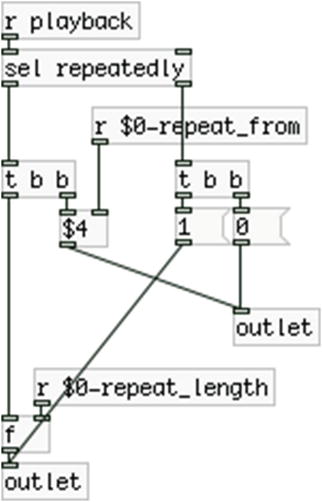
Figure 7-18. Contents of the $0-set_ramp_length subpatch
If we want to play a portion of the audio file, which we set with values from 0 to 1, we need to offset the ramp with the lowest value, and scale it with the difference between the two values, which is the value received by [r $0-repeat_length]. If, for example, we set to read the file from 0.25 to 0.60, we need our ramp to start at 0.25 and go up to 0.60, giving the ramp a total length of 0.35, which is the difference between the two values. This way we set the correct ramp for our sample without affecting the ramp that reads the smoothing window function. Of course, if we change the start and end point of the portion of the audio sample we want to play, [r $0-repeat_from] will receive the beginning point and store it in [$4 ]. If the Arduino sends any symbol other than “repeatedly”, we’ll send a 1 to [* ~], and a 0 to [+~ ], so we’ll multiply the ramp by 1, which gives the ramp intact, and we’ll add 0, which gives no offset.
This concludes the [read_samp] abstraction. It is a bit complex, but we’ll use it for all four sensors as is, the only thing we’ll change to each instance of the abstraction is its arguments. The next thing we need to do is build an abstraction to receive the input from the sensors, and that will be enough for our patch to work with the Arduino code. There will be only a minor addition to the Arduino code, which will enable us to control the threshold and debounce time from Pd, so we don’t need to upload the code every time we want to change one of the two values.
In the directory where you’ll save your main patch, make a directory called abstractions, and save [read_samp] in there. This abstraction is project-specific, so it’s better if you save it in a directory that’s not in Pd’s search path. (Don’t confuse the directory you’ll make and call abstractions with the abstractions directory that you might have already made and stored generic abstractions, like the ones from my “miscellaneous_abstractions” GitHub page. They should be two different directories in different places, even though they share the same name). In the main patch, we’ll use [declare] to help Pd find the abstraction.
Building the Abstraction to Receive Input from the Arduino
This abstraction is much simpler than the [read_samp] abstraction. It is shown in Figure 7-19. All we do here is receive input from a sensor and normalize its value to a range from 0 to 1, using the [map] abstraction. The values from the Arduino are printed with the “drum” tag along with the number of the pin of each sensor. In [drum] we have a [r drum$1]. This means that for the first sensor, we must provide the value 0 as the first argument to the abstraction, so that [r drum$1] will receive the value of that sensor. This abstraction has three inlets, one to set a new threshold, one to set a new debounce time, and one for debugging. The first two will take number atoms, while the third will take a toggle. When the toggle outputs 1, the value received by the sensor won’t go out the abstraction’s outlet, but will be printed as drum0, drum1, and so forth. This is very helpful as we can calibrate our patch on the fly. We’ll cover that a bit further on. When the abstraction outputs its value, it will send the normalized value out its right outlet and a bang out its left outlet, so it can bang [read_samp] and the patch will play the audio file.
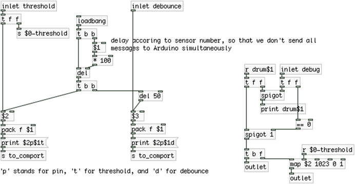
Figure 7-19. The “drum” abstraction
Sending the Threshold and Debounce Values to the Arduino
One thing we need to explain is the [loadbang] of the abstraction. Since we might want to have different thresholds and different debounce times for each drum, we need to set these as arguments and send them to the Arduino on load. To avoid sending all of these messages at the same time, we set a delay for each abstraction. This delay depends on the first argument of the abstraction, which is the number of the pin of the sensor each abstraction is listening to. So for the first abstraction, we’ll bang 0 × 100 = 0 milliseconds, so there’s no delay, and we’ll bang the threshold argument first, and the debounce argument delayed by 50 milliseconds. The second abstraction will have its arguments delayed by 1 × 100 = 100 milliseconds for the threshold argument, and another 50 milliseconds for the debounce. The third will be delayed 2 × 100 = 200 milliseconds, and so on. This way we avoid sending a bunch of messages all at the same time.
Lastly, I must explain the syntax of the messages sent to the Arduino. You’ve seen this in Chapter 2, but I’ll explain it shortly here as well. The message “print” sent to [comport] will convert all characters of the message to their ASCII values, which makes it easy to diffuse values in the Arduino code. To set the threshold for a specific sensor, we must define both the sensor pin and the threshold. The same applies to the debounce time. The message “print $2p$1t” will print the second value stored in [pack f $1], which is the number of the sensor pin, then “p”, then the value of the second argument, or the value sent in the leftmost inlet, and lastly, “t”. All numeric values will be assembled from their ASCII values in the Arduino code. When the Arduino receives “p”, it will set the value it assembled as the number of the pin. When it receives “t”, it will set the value it assembled as the value for the threshold for that pin. You’ll see that in detail when we go through the additions to the Arduino code.
Save this abstraction to the same directory with [read_samp]. You must have noticed that even though [read_samp] and [drum] are abstractions, we’re using hard-coded names for [send]s and [receive]s, like [s to_comport] or [r playback]. We should clarify the difference between a generic and a project-specific abstraction. When building generic abstractions (like [loop], for example), you should avoid using anything hard-coded; instead use rather flexible names (like [r drum$1]). Since these abstractions are meant to be used in many different projects, they should be built in such a way that they can adapt to any patch they’re used in. Project-specific abstractions are different because they are meant to be used in a single project, the one they are made for. In this case, it’s perfectly fine to use hard-coded names in [send]s and [receive]s, since that won’t create problems.
The Main Patch
Now that we’ve built the two abstraction we’ll need for our patch, it’s pretty simple to make the main patch. It is shown in Figure 7-20. In this patch, we can see the two abstractions we’ve made with their arguments. [drum] takes the sensor pin number, the threshold value, and the debounce time as arguments; whereas [read_samp] takes the name of the table where the audio file is loaded, the number of times the file is repeated when played in the ascending mode, the number of times it is played in the descending mode, the beginning and end of the repeated mode (in a scale from 0 to 1, where 0 is the beginning of the file and 1 is the end), and finally, the amount of time (in milliseconds) the file is repeated in the repeatedly mode.
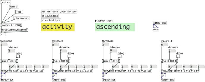
Figure 7-20. The main patch
Each abstraction takes a number atom for each argument to experiment with the playback settings and to calibrate each sensor. Notice that there’s a [r to_comport] which takes input from [s to_comport] which is in [drum], so we can send messages to the Arduino. Also notice that [drum] outputs the sensor value from its right outlet, which goes to [*~ ] to control the amplitude of the audio file playback, and it then bangs [read_samp] to read the file. We don’t need a [line~] to smooth the amplitude changes, because they occur before the file is triggered.
Apart from that we have a [declare -path ./abstractions], which tells Pd to look into the abstractions/ directory for the two abstractions. There’s also a [pd sound_tabs] subpatch. This is similar to the subpatch with the same name in Chapter 4, and it is shown in Figure 7-21. In this subpatch, we’re loading our audio files to the tables on load of the patch. The message to load an audio file is the same as already used in this book a few times. When [soundfiler] loads the file to the specified table, we convert its output (which is the length of the file in samples) to a bang so we load the next audio file. As you can see, I’ve made a directory called sounds in the directory of the main patch, and I’ve stored the audio files in there. Making separate directories for the audio files and the abstractions—instead of having everything together (along with the main patch) in the same directory—keeps things tidy and easy to understand.
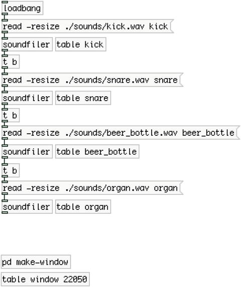
Figure 7-21. Contents of the sound_tabs subpatch
In [pd sound_tabs] there’s another subpatch, [pd make-window], which is shown in Figure 7-22. To avoid clicks, this subpatch creates the smoothing window we use for reading the audio files when the beginning and ending points are not zero. (Even if the beginning and end of the file are zero, when reading the file in the repeatedly mode, the two points will most likely not be zero, since we’ll be reading from some point other than the beginning to some point other than the end.) What this subpatch does is create a rapidly rising ramp from 0 to 1, taking 500 samples, then it stays at 1 for 21050 samples, and finally it makes a rapidly falling ramp from 1 to 0, which takes another 500 samples. You can see its output in Figure 7-23. We’re using [loop] to iterate through all the points of the table, and [moses] to separate the two ramps from the full amplitude value, 1. [moses] separates two streams of values at the value of its argument, or a value in its right inlet. Take a minute to try to understand how it works. The only thing that might be a bit confusing is [+ 499]. Since we start counting from 0, after 22050 iterations we’ll reach 22049.
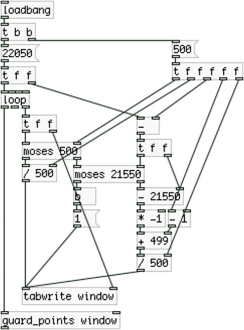
Figure 7-22. Contents of the make-window subpatch
Figure 7-23 illustrates what is stored in the window table. Its frame shows values between –1 and 1, in the Y axis, that’s why the window starts from the middle of the graph. You can see the rapidly rising ramp, which hits the ceiling of the graph when it reaches 1. It stays there for the greatest part of the table and it then goes back down to 0, making a sharp ramp. When we read each audio file, we’re reading this table at the same time and we’re multiplying the two tables. This results in beginning with silence, then rapidly rising to full amplitude, staying there for almost the whole table, and finally going back to silence. This prevents any clicks at the beginning and end points of the table, since they will always be silent.

Figure 7-23. The window table
Now I’ll explain [pd control_type], which is in the parent patch. This patch controls the two canvases, which label the kind of control that the foot switches have and the current type of playback. It is shown in Figure 7-24. This is an extremely simple subpatch, and we could have included these objects in the parent patch. It’s tidier and looks better if we place them in a subpatch. This subpatch takes input from the Arduino with the tags “control” and “playback”. The “control” tag inputs either a “playback” or “activity” symbol. The “playback” tag inputs “ascending”, “descending”, “backwards” or “repeatedly” .
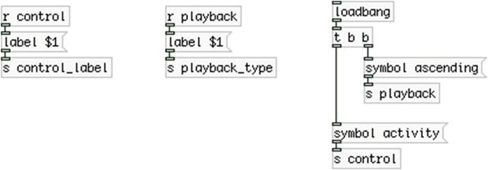
Figure 7-24. Contents of the control_type subpatch
The subpatch controls the label of the canvases in the parent patch, which on load are labeled as “activity” and “ascending”. “activity” is the default control of the switches when the Arduino starts. We explicitly set “ascending” as the default playback type. You need to set some of their properties to make it look like this. The Properties window of the “control” (the yellow) canvas is shown in Figure 7-25.
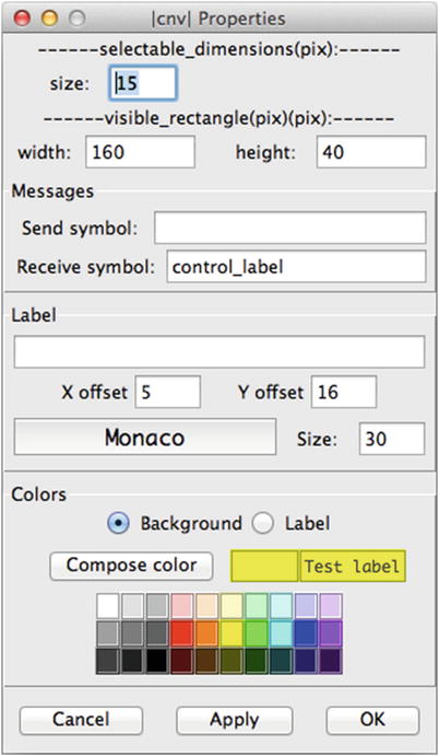
Figure 7-25. Canvas Properties
Change the Properties of the Playback Type Canvases
To open its properties right-click the top-left corner of the canvas, or left-click that point, and you’ll see a blue rectangle. That’s the control point of the canvas, which we can use to move the canvas around, or to open its properties. For this canvas, I’ve set its width to 160, its height to 40, its Receive symbol: field to control_label, which is the same name [send] has in Figure 7-24, its X offset to 5, its Y offset to 16, its Size: (this if the font size) to 30, and its color to yellow. To set the color, click the yellow square in the Colors field. This time we’re not controlling its color, or its size according to the messages we receive from the Arduino, like we did in Chapter 6. We’re only setting its label; that’s why we can set everything else using its properties, which is more user-friendly, than sending messages for each property. For the second canvas, the only differences are the width, which is 190, and the color, which is a default light green, from the squares in the Properties window.
Scaling the Output of the [read_samp] Abstractions in the Parent Patch
One thing that you might need to take care of is that the output of the [read_samp] abstractions is not scaled, so if you get two audio files being triggered simultaneously, or one triggered before the previous one has ended, and their amplitude sum is more than 1, you’ll get a clipped sound. Since this is aimed at being used with a drum set, you might set it up in such a way that you won’t have more than one audio file being triggered at a time. Also, the amplitude of the output of [read_samp] depends on how hard you hit a drum. For these reasons, I haven’t included any scaling to their output. It depends on your playing style and how you’re going to utilize this project, so have that in mind as you might need to apply some scaling to the output audio.
Finalizing the Arduino Code
Now that the Pd patch has been covered, let’s go back to the Arduino code to make the last additions. What we haven’t done yet is to allow Pd to control the threshold and debounce values for each sensor separately. Again, I’m not going to show the whole code, only the parts with the additions.
First of all, we now want to have separate threshold and debounce times for each sensor, therefore we need to create two new arrays for that, which are shown in Listing 7-8.
As you can imagine, these arrays will replace the two variables thresh, and debounce, which were defined in the beginning of the previous code, so make sure to erase them. Of course, these arrays need to be global, so place them before any function. I’ve placed them along with the rest of the arrays and variables for the sensors.
The next change occurs in the setup function, which is shown in Listing 7-9.
Since it’s not big, I’ve included the whole function to avoid any errors that could occur while adding things to the existing code. Here we’re just initializing the two new arrays with default values; all the values of the threshold_vals array are set to 100 and the debounce are set to 10.
The next addition is in the loop function, where we’re checking for input in the serial line and diffusing the values to their destinations. This is shown in Listing 7-10.
If there is data in the serial line, we’re creating two static ints, temp_val and pin, and then we’re checking what kind of input we got. If it’s numeric values we’re assembling them and store them to temp_val. If it’s ’p’, we’re copying the content of temp_val to pin and resetting temp_val to 0. If it’s ’t’, we’re assigning the value of temp_val to threshold_vals, to the element set by pin. Finally, if it’s ’d’, we’re assigning the value of temp_val to debounce, to the element set by pin. So if we send the message “0p150t” from Pd, we’ll store the value 150 to threshold_vals[0]. If we send the message “3p5d”, we store the value 5 to debounce[3]. This way we can dynamically set a new threshold and debounce time for every sensor individually. This means that whenever you use this patch and code, you should upload the Arduino code only once to your board, and then enable “debug” with the toggle in the [drum] abstraction. Then you should check each sensor by hitting the corresponding drum and make sure that you don’t get more than one value for each hit. If you get more than one, raise the debounce time. If you get only one, bring the debounce time even lower, until the lowest value that prints only one value per hit. The threshold will set how sensitive the sensor will be. This will also be helpful to avoid getting input from a sensor when you hit another drum, as your whole drum set may be vibrating and all the sensors might be giving output. You should bring the threshold to the lowest value where you get input from the sensor only when you hit the drum of that sensor. If you want your sensor to be less responsive, you should bring the threshold even higher. This type of control is very helpful because it enables the system to adapt to many different situations (different drum sets, different drum sticks, and so forth), without needing to tweak the code at all. If you want to save your new settings, all you need to do is change the arguments to the Pd abstractions.
The last addition to the code is in the for loop that goes through the sensors. The whole loop is shown in Listing 7-11 to avoid potential errors.
The only change is in line 4, where we now use threshold_vals[i] instead of thresh, and in line 22, where we use debounce[i] instead of debounce. Using arrays enables us to have a different value for each sensor, which gives us great flexibility. And this concludes the code in this project. Make sure that you’ve written everything correctly, and that your code and patch work properly. Once you have everything working as expected you can start building your circuit on a perforated board and enclose it in a box. Next, I’ll provide some suggestions on how to make an enclosure to keep your project safe for transporting, and easy to carry and install anywhere.
Making the Circuit Enclosure
Bringing around a circuit on a breadboard is not really a good idea, because every time you’ll probably need to build the circuit from scratch, as the breadboard is not stable and the circuit can get destroyed during transfer. The breadboards are designed only for testing circuits. What’s best is to build the circuit on a perforated board and close it in a box so you can easily carry it around. Another good idea is to build your sensors in such a way that it’s easy and safe to carry them around. Figure 7-26 shows a piezo element connected to a mono 1/8-inch jack. This way it’s very easy to transport them and use them.
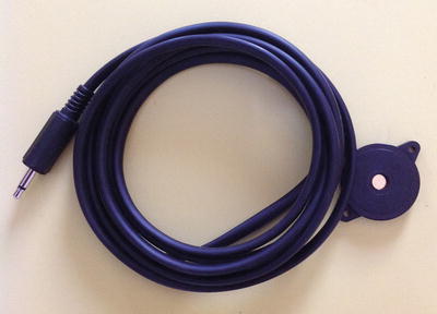
Figure 7-26. Piezo element wired to a 1/8-inch jack
Figure 7-27 illustrates a box that I have made for this project. On the front side, there are four quarter-inch female jacks for plugging in the foot switches, which usually come with a 1/4-inch male jack extension. Since the switches have two pins, these jacks are mono. On the top side of the box, there are the four LEDs that indicate which sensor is active and which is not, and the four female 1/8-inch jacks for the sensors. This setup makes it extremely easy to plug in your switches and sensors, and play.
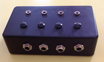
Figure 7-27. Box containing the circuit of the project
This box doesn’t contain an Arduino, but it has a IDC male angled connector on its back side, which you can see in Figure 7-28. I’ve used a Proto Shield along with the Arduino, which makes prototyping very easy, giving easy access to all the pins of the Arduino.
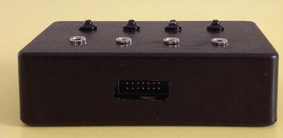
Figure 7-28. Back side of the box
To connect the box to the Arduino I just used a ribbon cable (the kind of cable used with the IDC connectors) between it and the Proto Shield. You can see that connection in Figure 7-29.
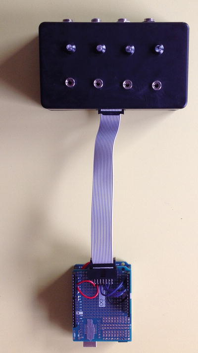
Figure 7-29. Connecting the circuit box to the Arduino
What you need to take care of is how you’ll wire both the circuit board and the Proto Shield. First, connect the two IDC connectors and then check which component is connected to which pin of the IDC, so that every component goes to the correct pin. IDC connectors may be a bit confusing, and you’ll probably need a multimeter to use its continuity to verify your connections. You’ll also probably need to solder some wires on the back side of the circuit board and the Proto Shield.
I’ve already mentioned that when building circuits, it may be preferable to have only one component connected to ground on the circuit board, and pass it to the other components (the same goes for voltage, but we’re not passing voltage here). Here, I have connected the first 1/4-inch jack to ground and I have then daisy chained all components. Another thing I have used is stereo female 1/8-inch jacks for the piezo elements. Even though they require mono jacks, using stereo in the box makes it easier to pass the ground to the other components. As soon as you connect the male mono jack, the first two pins of the stereo female jack will be connected (it’s pretty simple why this happens, test for yourself with a multimeter). This way you can use one pin to receive ground from the previous component, and another pin to pass the ground to the next component. You could apply this to the 1/4-inch female jacks too.
Another thing that you might want to consider is to minimize the components on the circuit board as much as you can. In the same line of using the integrated pull-up resistors of the Arduino, you can solder the other resistors right on their components. Figure 7-30 shows how I soldered the 1MΩ resistors of the piezo elements on the female 1/8-inch jacks.
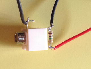
Figure 7-30. 1MΩ resistor soldered on a 1/8-inch female jack. The first two pins are used to receive and pass ground
Soldering these resistors on the jacks is pretty easy (this is another advantage of using stereo female jacks with mono male jacks) and minimizes the circuit you need to solder on the perforated board. In Figure 7-30, you can also see how the stereo jack is used to easily receive and pass ground. When a mono male jack is inserted, the two wires on top are both grounded, since they both touch the same area of the male jack. The left one receives ground from the previous component, and the right one passes it to the next component. Mind, though, that this is true only when the male mono jack is plugged in. If you don’t plug in a mono male jack, the two pins won’t be connected. If you plug in a stereo male jack, again the two pins won’t be connected, because they will be touching different parts of the male jack. If you omit connecting a piezo element, make sure you don’t have any other components in the chain waiting to receive ground; otherwise, any components after the unconnected female jack won’t be grounded and won’t work. You can also wire the 220Ω resistors of the LEDs on their long legs, but I didn’t do that. I prefer to solder these resistors on the perforated board instead.
On the one hand, this kind of enclosure makes the circuit very stable, easy to use, and safe to transfer; on the other hand, you don’t need to “sacrifice” your Arduino since you’re not enclosing it along with the circuit, enabling you to use it for other projects any time.
Conclusion
We have created a robust and flexible combination of hardware and software that enables us to extend the use of the drums. As with all projects, the Pd patch is only a suggestion as to what you can do with these sensors. You can try out different things with this patch and build something that suits your needs. The Arduino code is not so much of a suggestion, as it provides a stable way for these sensors to function as expected. This also applies to the part of the Pd patch that reads the sensor data (the [drum] abstraction).
The threshold values used here are most likely very low, and you’ll probably find that you need much higher values to avoid getting input from one sensor when you hit the drum of another sensor. A very low threshold might also result in getting more than one value per hit, even if you use a rather high debounce time value. Setting these two values is a matter of personal playing style, what you actually want to achieve, and the drum set you use.
Another thing to bear in mind is that you might not want to use sensors on drums that share the same base (tom drums, for example, which are based on the kick drum). Also, depending on the tuning of the drums, hitting a drum might cause another drum to resonate, which can also be a factor you’d like to experiment with. Regardless of these aspects, your sensor setup should bring in a lot of inspiration and fun.