In the previous chapter, we saw how to run queries that will return data that you need. This chapter will cover what happens behind the scenes when you run such queries and how the database executes them. We will also show some challenges database needs to solve and how databases are coping with ever-growing data. This chapter will present some possible optimization solutions. Finally, we will show how RavenDB prevents common problems with queries.
Queries from the Perspective of a Database
As users and developers, we execute queries against the database to get results back. This action is so standard that we do not think about underlying mechanisms and tools that deliver results. Additionally, working with a relational database, you probably use Object-Relational Mapper, representing an additional layer of abstraction between your code and a database. Over time, as we work with databases, we tend to forget what happens behind the scene.
Unbounded Queries
Unbounded query over Employees collection
The database engine will fetch all employees from the disk and return them. Unbounded queries can be dangerous, as things are not under your control. Results of execution are not deterministic, but they depend on the number of documents. If we are processing employees, we do not know if we will iterate over 10 or 10,000 employees. Furthermore, for all visual representations of our company employees, we will rarely need all of them .
Paging
so query from Employees limit 0, 2 will return first two employees.
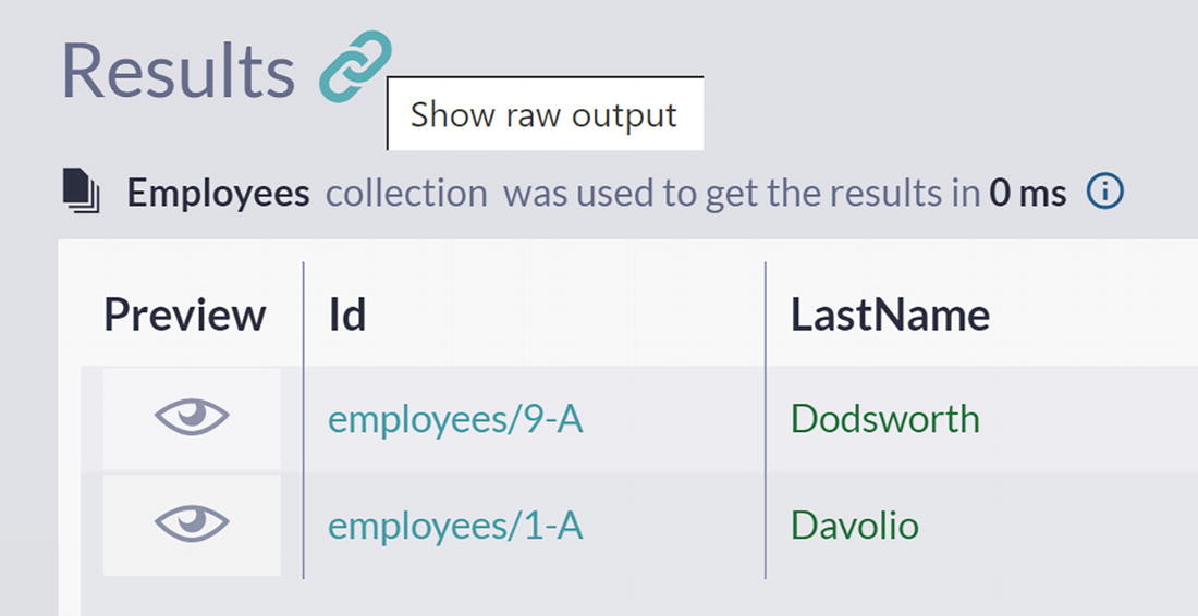
A screenshot of the results panel with a chain icon and a text box next to it has text show raw output. A table with 3 columns, preview, I d, and lastname is listed under the index employees.
Show Raw Output Icon
The client interprets this response, in this case, RavenDB Studio, to show you query results. Not all properties of returned JSON are rendered in Studio – as you can see, the first property contains a total number of results. So, you can display the total number of results in paged query with just one request to the server .
Filtering
The query for employees living in London
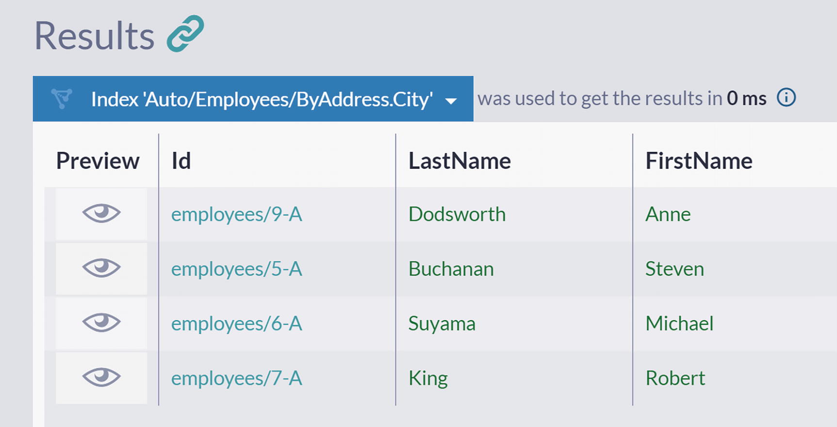
A screenshot of the results panel in the query window under index auto slash employees slash by address dot city. A table is listed with the columns, preview, I d, last name, and first name.
Employees Living in London
As you can see, the engine managed to find those living in London. So, if you had to perform the same task, how would you do it?
Let’s imagine that you have nine papers representing each of the employees. Taking one by one, you would look at the Address, checking if City is London. If this is the case, you will stack paper to the right. Otherwise, you would put it to the left. After you process all documents, the stack to the right will contain all four employees living in London.
What you just did is very similar to what a database engine might do in some cases, and it is called sequential scan or full table scan. It might seem like a logical move at first sight. However, what happens as the number of employees grows in your database? Or, if you filter orders in a retail operation, you have thousands and thousands of orders after a couple of years. How long will it take to filter orders by some of their properties? No matter how fast the disk or CPU, your application will start suffering from a full table scan sooner or later.
In algorithmic complexity terms, this operation has O(n) complexity – if you increase the amount of data ten times, filtering will take ten times longer. It is evident that this approach is not a sustainable one and that we need a different one. However, no matter what method we use, the database engine still needs to visit every employee to check the living city .
Indexes
So, if we cannot eliminate this sequential scan, one conceptual solution would be to perform it once and save results for subsequent calls. This approach is how all modern databases are solving this challenge. You can specify a field, and the engine will go over all documents looking at the content of this field. Discovered values will be stored in a particular data structure called Index. An index is an additional data structure (metadata, or “data about your data”) stored along with your documents. The database will derive the content of the index from your content, and it will never alter it.
In our example, we would define index over Address.City field of an Employee document, and we would say that this field is indexed. When computing the content of this index, the database would extract all distinct values (all cities) and store them in a specialized data structure. Various indexing structures were developed over the years, but all of them have a clear purpose – to provide a fast way to fetch documents based on some criteria.
Content of Employee.Address.City Index
Address.City | ID |
|---|---|
Kirkland | employees/3-A |
London | employees/9-A employees/5-A employees/6-A employees/7-A |
Redmond | employees/4-A |
Seattle | employees/1-A employees/8-A |
Tacoma | employees/2-A |
Obtaining a list of all employees from London is now easy. Their identifiers will be collected, and those documents will be fetched from the disk and delivered. You could say that we prepared ahead of time for all possible Address.City queries. We precomputed results and stored them side-by-side with documents. As a result, our queries will be fast. There are no more table scans: no more need to go over documents and load them to check if they should be included in the result set. We have a list of IDs that can be read directly from the disk, with certainty that this is a complete result set.
Types of Indexes
If a computation is inevitable, there is no way to avoid performing it. However, you can do it just once and save results to a disk ahead of query time. Indexes are precomputed answers stored in a specialized data structure that provides a fast way to fetch results .
In Table 4-1, we presented an index that contains document IDs. Such an index is called the secondary index .
When a secondary index is used to service a query, one more step is needed before the list of employees is returned to you. The database needs to use IDs obtained from the secondary index to fetch complete employee documents. This operation needs to be efficient, so the database will maintain one more index that tracks the exact storage position of each document based on its identifier. This index is called the key-value index , and if you have been working with relational databases, you will recognize a similar internal data structure as the primary index .
Overall, a query like Listing 4-2 will require a database to perform two operations. First, taking the value of an indexed property, a secondary index will be consulted to obtain a list of identifiers. Second, the primary index will be used to fetch employee documents from database storage efficiently.
Content of Clustered Index
City | ID | Document |
|---|---|---|
Kirkland | employees/3-A | {id: “employees/3-A”, ”FirstName”: “Janet”..} |
London | employees/9-A employees/5-A employees/6-A employees/7-A | {id: “employees/9-A”, ”FirstName”: “Anne”..} {id: “employees/5-A”, ”FirstName”: “Steven”..} {id: “employees/6-A”, ”FirstName”: “Michael”..} {id: “employees/7-A”, ”FirstName”: “Robert”..} |
Redmond | employees/4-A | {id: “employees/4-A”, ”FirstName”: “Margaret”..} |
Seattle | employees/1-A employees/8-A | {id: “employees/1-A”, ”FirstName”: “Nancy”..} {id: “employees/8-A”, ”FirstName”: “Laura”..} |
Tacoma | employees/2-A | {id: “employees/2-A”, ”FirstName”: “Andrew”..} |
The database engine can fetch the list of employee documents with just one round trip to the storage with a clustered index. Unfortunately, such an index is expensive storage-wise since it will essentially duplicate all records from the primary data storage into metadata structure. Various relational databases are using different approaches to overcome this challenge. SQL Server allows just one clustered index per table; MySQL is implementing primary index as clustered, with secondary index entries pointing to primary keys.
Content of Covering Index
Address.City | ID | FirstName |
|---|---|---|
Kirkland | employees/3-A | Janet |
London | employees/9-A employees/5-A employees/6-A employees/7-A | Anne Steven Michael Robert |
Redmond | employees/4-A | Margaret |
Seattle | employees/1-A employees/8-A | Nancy Laura |
Tacoma | employees/2-A | Andrew |
Covering index is a compromise that enables the database to answer some of the queries using index alone (hence the term covered, since such index covers some of the queries) without allocating too much space .
Downsides of Indexing
Indexes sound like a great idea, but there are also downsides. Storing additional data structures on the disk will inevitably take extra space. In our example, we defined the index on just one field of the Employee document. If we wanted to provide users with efficient filtering on other fields like FirstName or LastName, we would have to expand EmployeeIndex with entries for these two fields. Over time, as you define new indexes, expand existing ones with additional fields, and increase the number of documents in your database, the total size of indexes will inevitably grow, allocating more and more space for this metadata.
However, there is another much more challenging task – index maintenance. Every time we update an employee’s city of living or any other indexed field, we need to update the Index. Every time we create a new employee in the database, the Index needs to be updated. As a result, each write to a database will be accompanied by additional one or more index update operations. Both of them, writing data and index updates, will be performed together, making your writing operation slower.
This results in an interesting trade-off: we will introduce indexes to speed up queries , but these will slow down writes. We want to have fast queries, but at the same time, we do not want to slow down writes. Hence, we should carefully select which fields should be indexed based on the applications’ usage patterns. This trade-off explains why databases are not indexing everything by default – this approach would introduce unnecessary overhead.
Even though querying via indexes (opposed to querying raw data) is what every developer should be doing, a lack of indexes is probably the most common anti-pattern among programmers. There are various contributing factors to this sad fact, but the need for the manual creation of indexes is the most significant one. It is easy to forget about it or make an omission, even when you are informed and aware. Additionally , this mistake is usually well-hidden in a small amount of data. Developers testing an application on a small dataset will not experience the dreadful consequences of a full table scan. Without load testing, a developer will deliver the database without indexes to production.
Eventually, a lack of indexes will result in a significant and annoying slow-up of the application. With the small amount of data in the database, the application will be fast, but over time, as the amount of data grows, performance will start to degrade linearly. This gradual degradation is a severe obstacle to the scaling of your application and will make you go back and fix performance problems, which will cost you both time and money .
RavenDB’s Indexing Philosophy
The general philosophy of RavenDB design as a database is not to help you solve problems and challenges but to prevent them. This approach has unique consequences – your database will make bad things impossible, or when you make an omission, RavenDB will react and correct your actions.
As a part of this prevention philosophy, in RavenDB, all queries are always executed via indexes. It is technically impossible for a query to avoid execution via index. This way, the manual omission is not possible, and all filtering queries will be efficient.
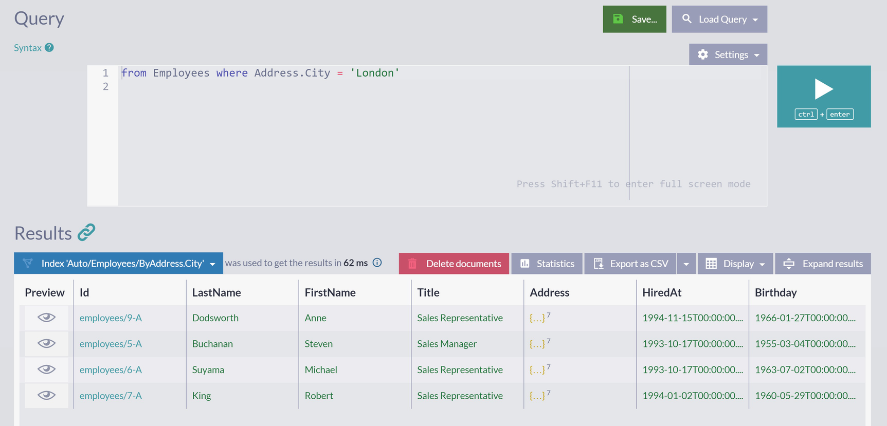
A screenshot of the query window with a save button, search box, and settings drop-down list. A query reads from employees where address dot city equals London. The results panel has a table with 8 columns.
Results Panel
Not only that an error was not displayed, but we also got the actual result set. How come?

A screenshot of the results panel for index auto slash employees slash by address dot city with the execution time of 62 milliseconds. A table has 4 column headings only namely preview, I d, last name, and first name.
Index Details
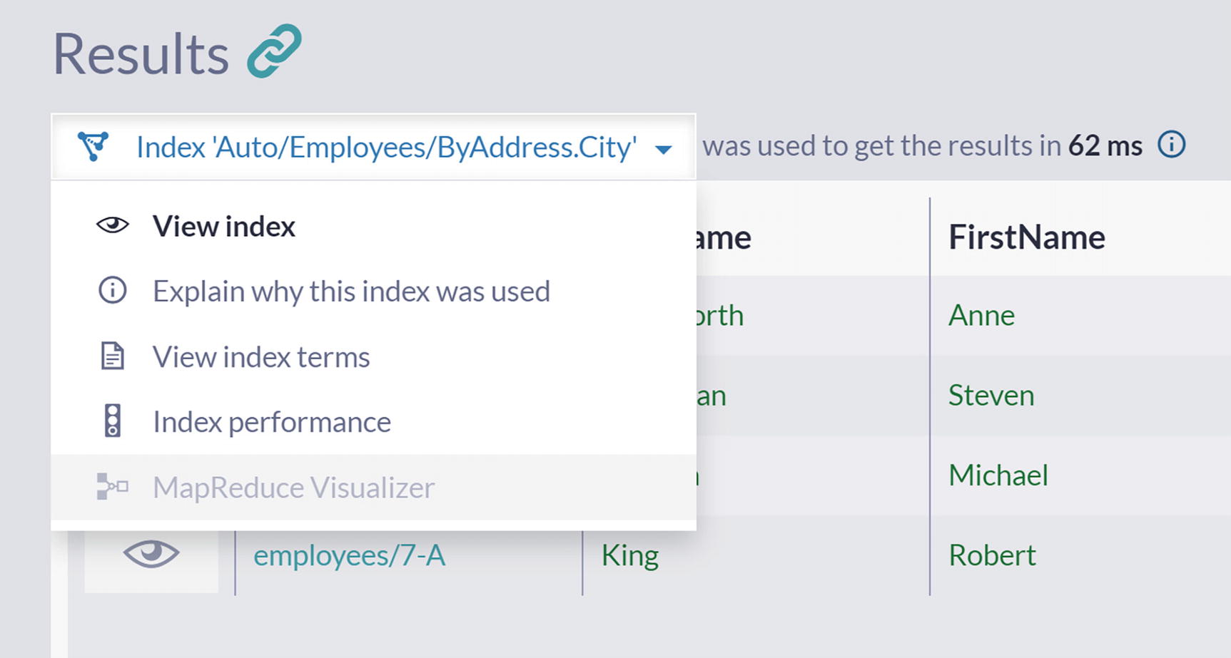
A screenshot of the results panel in the query window with index auto slash employees slash by address dot city in the drop-down menu of 5 options. A table with 4 columns is listed in 62 milliseconds.
View Index Option
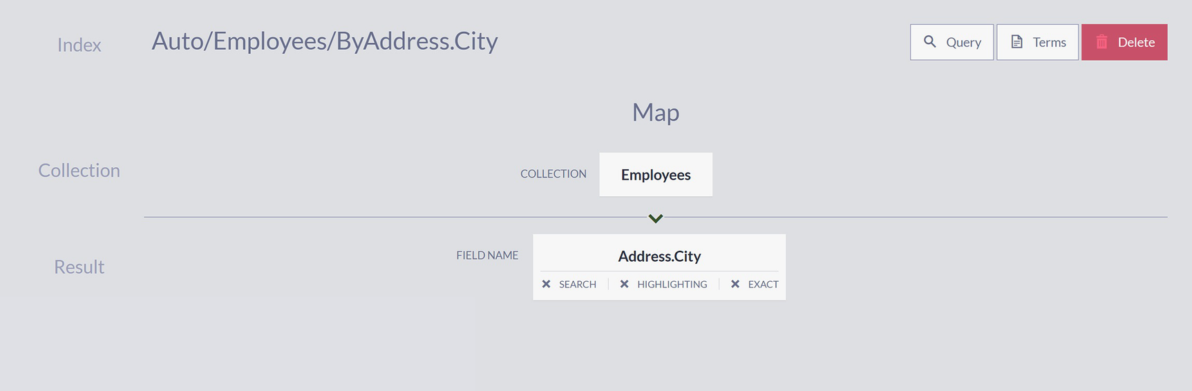
A screenshot with data auto slash employees slash by address dot city on index, employees on collection field, and address dot city on field name with options query search, terms, and delete button.
Structure of Index

A screenshot depicts the index terms for auto slash employees slash by address dot city with 2 sections namely address dot city and i d.
Index Terms
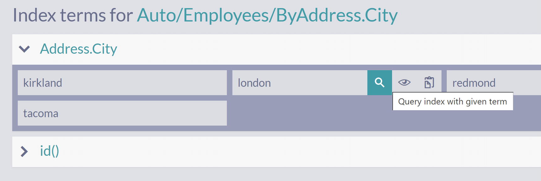
A screenshot depicts the index terms for auto slash employees slash by address dot city with 2 sections, i d and address dot city that displays 4 cities that are Kirkland, London, Redmond, and Tacoma.
Querying over Index Terms

A screenshot of the query window depicts 2 panels, search query, settings menu, and save and play buttons. A query reads auto slash employees slash by address dot city where address dot city equals London. The results panel at the bottom has a table with 11 columns.
Results of Executing Query over Index
As observed in Figure 4-9, we are now querying the index directly, and the results are the same as when we executed the query from Listing 4-2. This is expected since the same index was used when we queried the collection directly.
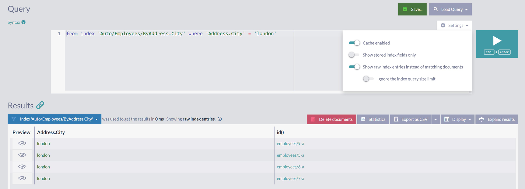
A screenshot of the query window depicts 2 panels, settings drop-down menu with 4 toggle buttons, search query, save, play, and delete buttons. The top panel contains a query and the results panel at the bottom has a table with 3 columns.
Raw Index Entries
Looking again at Table 4-1, we can see that this is the precisely same set of entries for “London.” Modifying this query and running it for the rest of the cities from Figure 4-8 will return the remaining items from Table 4-1.
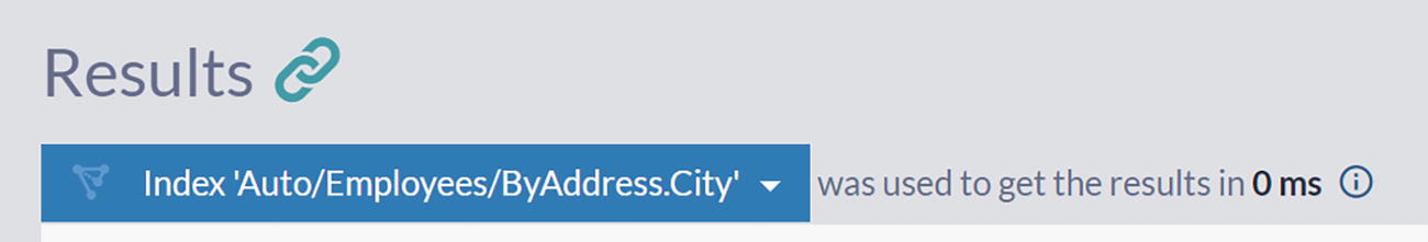
A screenshot of the results panel in the query window with a chain icon depicts the index auto slash employees slash by address dot city in the drop-down menu with the execution time of 0 milliseconds.
Query Execution Time
We did not mention it earlier, but this Query execution time measures server-side execution time. Even if you experienced a long time waiting for results to appear in your browser, you were waiting for the result set to be delivered to your browser. The measurement shown here is the actual time it took the database to generate these results.
Comparing query timing for this attempt with the previous one from Figure 4-3, you can see that we are much faster this time. On the first run, after failing to find an appropriate index, RavenDB had to create one. This operation took some time – the database had to fetch all nine employees from the disk, process their Address.City field, extract values, and form an index out of those values.
On the second run that we just did, a suitable index was detected right away and used to deliver results. The same scenario will happen on any subsequent run – precomputed values will be read from the disk and returned .
Summary
In this chapter, we introduced the concept of an index as a specialized data structure. An index is metadata placed side by side with your data inside a database, and it is one of the possible solutions for speeding up queries. We showed how RavenDB’s design approach would help you prevent common problems with indexes.
In the next chapter, we will show how you can control index creation and define it yourself instead of letting RavenDB create them automatically.