© The Author(s), under exclusive license to APress Media, LLC, part of Springer Nature 2022
D. MiličićIntroducing RavenDBhttps://doi.org/10.1007/978-1-4842-8919-8_6

6. MapReduce Indexes

Dejan Miličić1  
(1)
Novi Sad, Serbia
 

The previous chapter demonstrated complete control over an index’s definition and life cycle. Map and MultiMap indexes were introduced, along with various ways to compute fields that can be used to filter and sort documents. This chapter will show how to perform grouping and aggregation in RavenDB. Concepts of MapReduce and MultiMapReduce indexes will be introduced, along with a way to materialize the content of the index into a new collection.

Grouping

Queries executed in the previous chapter were about filtering. The filtering condition was defined, and the database returned all documents that matched it. Typical queries of this kind look like this:
from index 'Auto/Employees/ByFirstName'
where FirstName = 'Nancy'
or
from index 'Orders/ByEmployeeNameByTotal'
where Total > 15000
Besides filtering documents, RavenDB is also capable of grouping data . Let’s say that we would like to analyze Orders by the shipping country. You can achieve that by running the query shown in Listing 6-1.
from Orders as o
group by o.ShipTo.Country
select o.ShipTo.Country
Listing 6-1

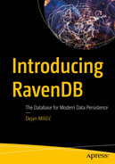
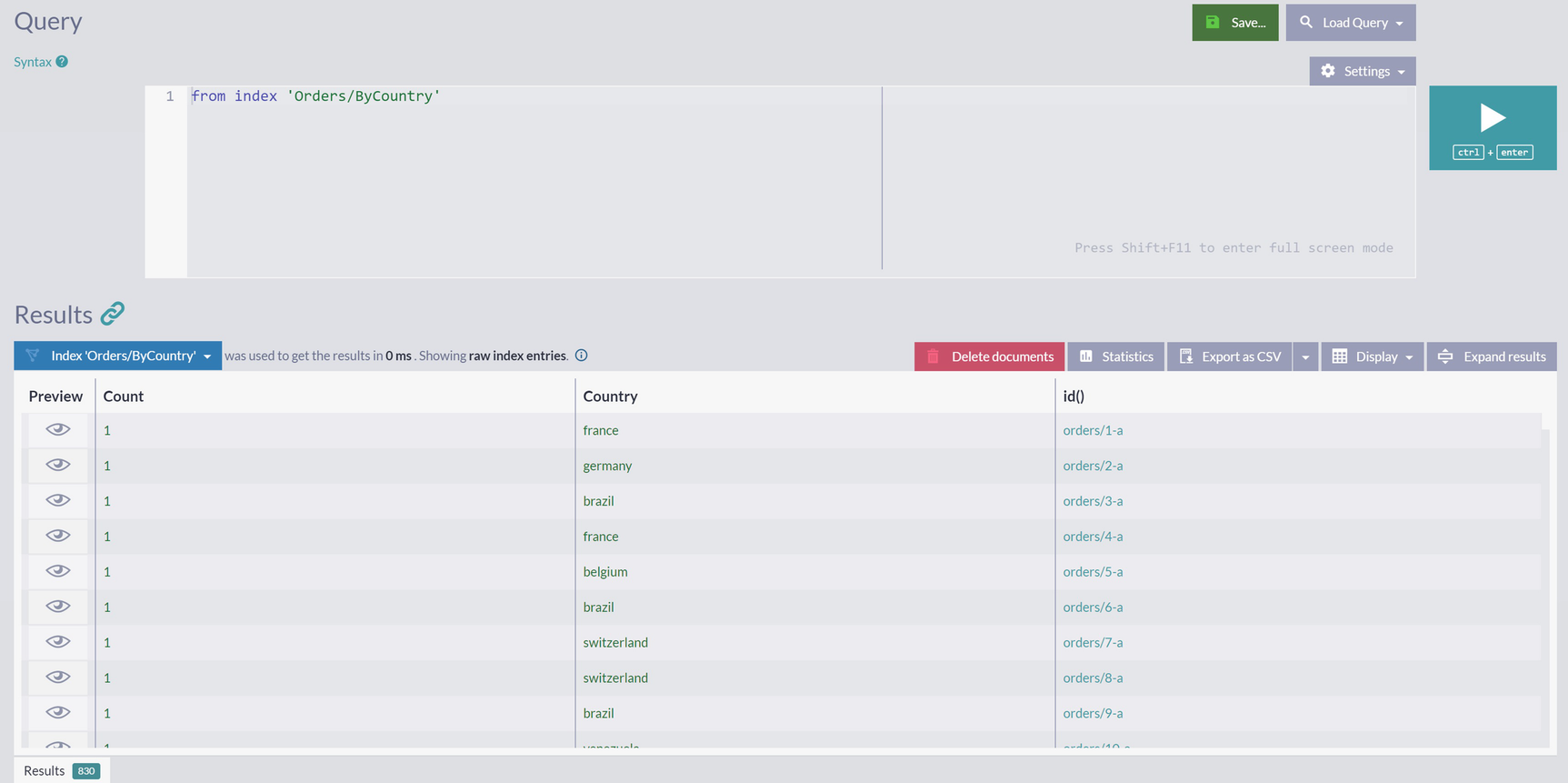
Grouping orders by the country of shipment

This query will result in a list of 21 different countries Northwind Traders sent orders to, as shown in Figure 6-1.

A snapshot of the query result of a list of 21 countries. France, Germany, Belgium, Brazil are some of the countries in the list.

Figure 6-1

Shipping Countries for Orders

As with all previous queries you saw, this one also uses an index to return results. Since we did not define static one upfront, RavenDB created the automatic index Auto/OrdersReducedByShipTo.Country which is visible in the listing of all indexes for your database. Clicking on it will reveal index details shown in Figure 6-2.

A snapshot of all indexes database for the country available in the database.

Figure 6-2

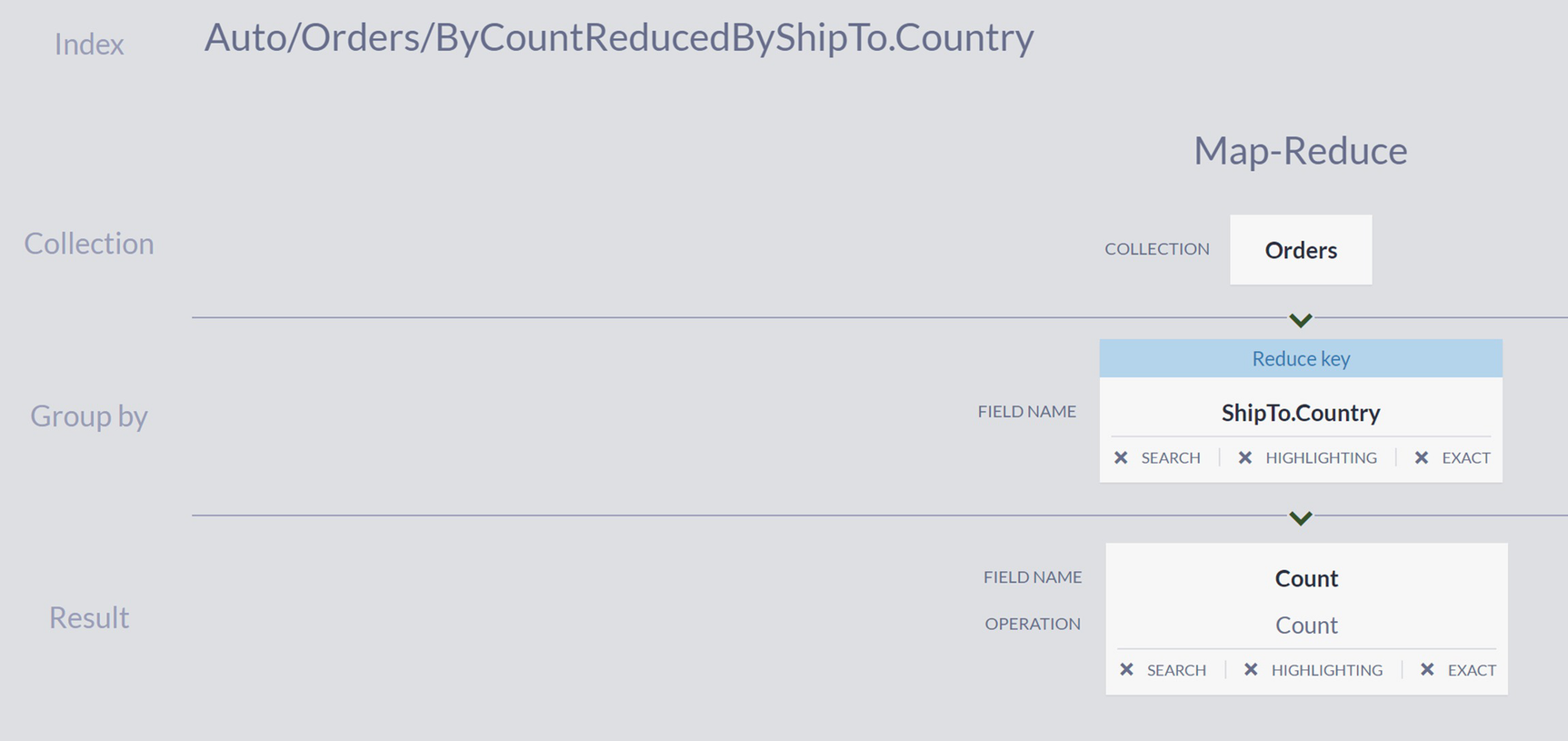
Structure of Auto Index Auto/OrdersReducedByShipTo.Country

Documents from Orders collection were processed, their ShipTo.Country values were extracted, and IDs of orders with the same values were stored in index entries. RavenDB uses a specific programming model we will examine in the next section for processing grouping tasks .

MapReduce

Figure 6-2 displays a visualization of the data grouping pipeline in an index. At the top of this diagram, you will see the Map-Reduce heading, denoting this index type. Alternatively spelled as MapReduce, this technique popularized by Google is used for the parallel processing of data across many machines. In a typical setup, data is first split into batches. Every batch is sent to a different device, which will use the map function to transform all entries in the received collection. Mapped entries are then combined via reduce function to produce the final result set.

The previous chapter saw examples of automatic and static indexes implementing map functions to transform documents into indexing entries. MapReduce index will take such mapped entries and apply reduce function to them, emitting grouped entries. RavenDB is using a variant of this programming model.

Unlike original MapReduce used at companies like Google, where data batches are distributed across hundreds and thousands of machines, RavenDB performs this process on a single machine. Multiple threads will receive packs, apply map function to emit projections first, and then apply reduce function to these projections.

RavenDB has a MapReduce visualizer that can help you examine MapReduce indexes. You can open it by clicking on the Indexes option in a sidebar, then the Map-Reduce Visualizer option, as shown in Figure 6-3. Understanding this process can be a bit tedious if this is the first time you are working with MapReduce or when you want to debug results over a large amount of data.

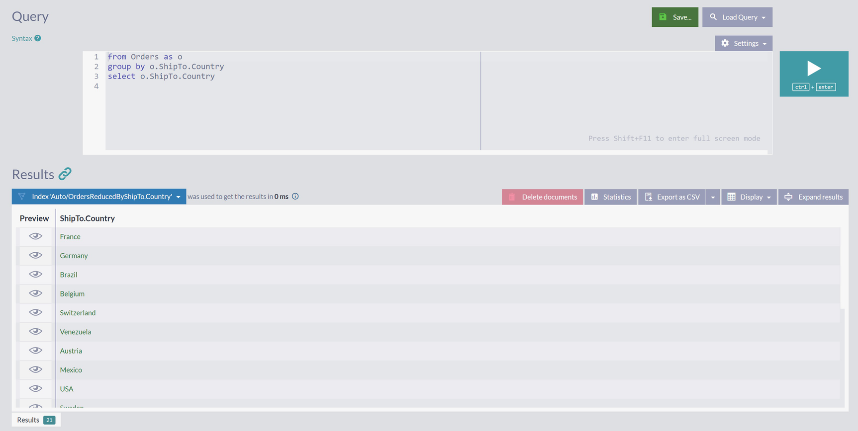
A snapshot of the selecting index, entering documents, area of interest, and map-reduce details options for the map-reduce menu.

Figure 6-3

Map-Reduce Visualizer Initial Screen

On this screen , you can select the index your query created a moment ago, Auto/OrdersReducedByShipTo.Country, and select documents to present visualization for. Selecting orders/1-a and orders/103-a will generate representation as in Figure 6-4.

A snapshot of the orders being ready to ship to France.

Figure 6-4

Map-Reduce Visualization of Auto/OrdersReducedByShipTo.Country Index for orders/1-a and orders/103-a

Map phase of the index extracted ShipTo.Country, while Reduce phase collected all orders with same shipping country. In Figure 6-4, you can see that the reduction phase gathered these two orders together since their shipping countries match. If you check the documents for these two orders, you will know that they went to France.

Clicking on the reduction box will expand the tree’s root, as shown in Figure 6-5.

A snapshot of the tree roots expansion for the two orders.

Figure 6-5

Reduction Outcome Details

You can see that the reduction phase grouped numerous orders shipped to France and that the two orders we selected are just two of many such orders. Clicking on the reduction box will show a scrollable listing of all these orders, as shown in Figure 6-6.

A snapshot of the scrollable listing of all the orders.

Figure 6-6

Reducing Orders Shipped to France

The ability for a database to perform groupings like this one is nice, but it is not too valuable. The full power of grouping comes with aggregation, which we will cover in the next section.

Aggregation

We started this chapter with a query shown in Listing 6-1. When executed, it will produce a list of shipping countries. However, we would like to see how many orders are shipped to these countries. Query returning that info is shown in Listing 6-2.
from Orders as o
group by o.ShipTo.Country
select o.ShipTo.Country, count()
Listing 6-2

Grouping and counting orders by the country of shipment

If you compare Listing 6-2 with the previous query in Listing 6-1, you can see that we expanded the select statement with count(). This query expansion will result in the addition of results, as shown in Figure 6-7.

A snapshot of the shipping countries and their order counts.

Figure 6-7

Shipping Countries for Orders Expanded with Count

Counts shown are calculated by applying the process of aggregation – calculating combined values for a group of results. In this case, RavenDB counted one for every order in a country group and came up with a total sum. Finally, we can execute this query:
from Orders as o
group by o.ShipTo.Country
order by count() as long desc
select o.ShipTo.Country, count()

and obtain a piece of useful information regarding the “Northwind Traders” business – most of their orders, 122, were delivered to customers in the United States and Germany.

As you can see, this query created the new automatic index Auto/Orders/ByCountReducedByShipTo.Country, and clicking on its name in the list of all indexes will reveal its internal structure, as shown in Figure 6-8.

A snapshot of the collection, group by, and result of the orders reduced.

Figure 6-8

Structure of Auto/Orders/ByCountReducedByShipTo.Country

If you compare this with Figure 6-2, you can see that the original automatic index was augmented with count operation in the aggregation phase.

Examining indexing terms for this index reveals fields with names Count and ShipTo.Country. These two aggregation categories provide us with a way to find out how many shipments went to Finland :
from index 'Auto/Orders/ByCountReducedByShipTo.Country'
where 'ShipTo.Country' = 'finland'
or to get a listing of all countries with more than 80 orders shipped to
from index 'Auto/Orders/ByCountReducedByShipTo.Country'
where 'Count' > 80

Static MapReduce Indexes

The previous chapter introduced the concept of static Map indexes . They are a natural extension of Map indexes, providing a way to map documents and then specify how to aggregate those maps. It is also possible to write static MapReduce indexes. This section will recreate a static version of automatic index Auto/Orders/ByCountReducedByShipTo.Country.

Start by creating map index, as shown in Listing 6-3:
map("Orders", order => {
    return {
        Country: order.ShipTo.Country
    }
})
Listing 6-3

Orders/ByCountry map index

This index is not much different from the Employees/ByFirstName index in the previous chapter – for every order document, RavenDB will create one indexing entry with Country value.

Final goal of this static index is to count totals, so let’s expand mapping with numbers that you will aggregate later on, as in Listing 6-4:
map("Orders", order => {
    return {
        Country: order.ShipTo.Country,
        Count: 1
    }
})
Listing 6-4

Expanding Orders/ByCountry map index with count

Raw indexing entries for such expanded map index can be found in Figure 6-9.

A snapshot of the index orders by countries.

Figure 6-9

Raw Indexing Entries for Expanded Map Index Orders/ByCountry

This index is now performing the same task that you would do manually – going one by one order and writing down every occurrence of each country from ShipTo.Country field. After writing down marks of this kind for all orders, you would go back and sum it up. And that is precisely what the reduction phase of the MapReduce index does.

To add reduction script, open index for editing and click on Add Reduction button. New panel will open and you can add JS code for reducing all mappings that are emitted by map function. Code for this is visible in Listing 6-5:
groupBy(map => map.Country)
    .aggregate(group => {
        var country = group.key;
        var count = 0;
        group.values.forEach(el => {
            count += el.Count;
        })
        return {
            Country: country,
            Count: count
        }
    })
Listing 6-5

Reduction code for index Orders/ByCountry

Figure 6-10 shows the final form of the Orders/ByCountry MapReduce index .

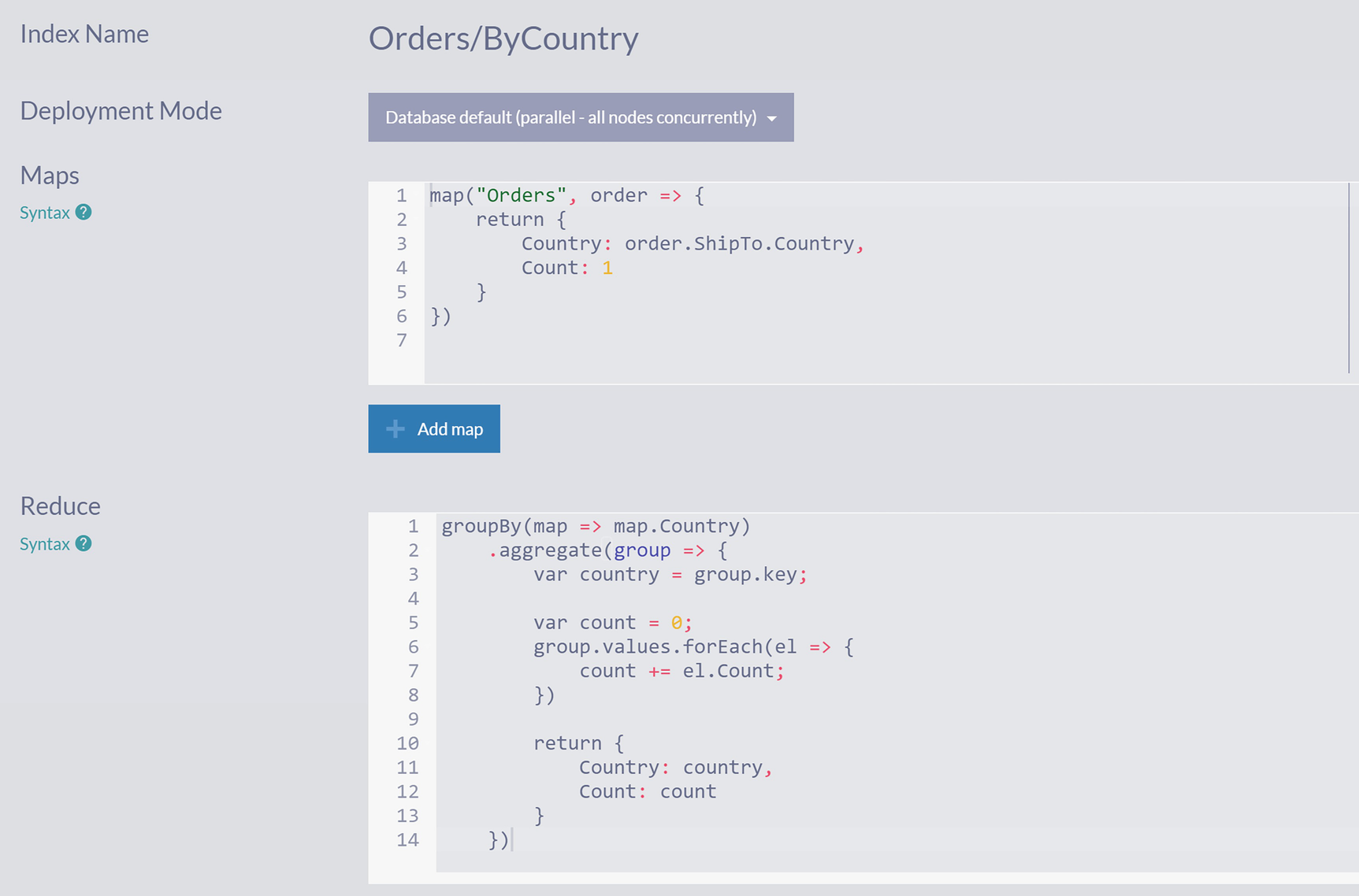
A snapshot of the code for the orders by country.

Figure 6-10

MapReduce Index Orders/ByCountry

Reduce script from Listing 6-5 can be refactored. Refactoring is the process of changing implementation without changing behavior. Let’s reorganize the code to make it more concise.

First, you can replace imperative forEach loop defined in Listing 6-8 with functional equivalent based on reduce function:
groupBy(map => map.Country)
    .aggregate(group => {
        var country = group.key;
        var count = group.values.reduce((res, el) => res + el.Count, 0);
        return {
            Country: country,
            Count: count
        }
    })
Reduce method may look strange, but it is the declarative equivalent of an imperative for loop. It operates on arrays in JavaScript and has the following form:
array.reduce(reducer, initialValue);
Reduce method starts with initialValue (in our case, zero) and then applies reducer action over all elements of an array. You can think of a reducer this way:
reducer(result_from_previous_call, arrayElement) => new_result
In the first application, there is no result from the previous call, so that initialValue will be used, and the first element of the array will be consumed, resulting in
var res0 = reducer(0, arr[0])
After that, the next array element will be processed:
var res1 = reducer(res0, arr[1])

This process will continue until all array elements are processed. Hence, we iterated over all array elements in a recursive declarative way.

Reducer function itself is simple addition of two arguments:
reducer(accumulatedValue, el) = accumulatedValue + el.Count
As a second and final step in refactoring of reduction phase of our index, you can inline country and count variables:
groupBy(map => map.Country)
    .aggregate(group => {
        return {
            Country: group.key,
            Count: group.values.reduce((res, el) => res + el.Count, 0)
        }
    })
At this point, the automatic index Auto/Orders/ByCountReducedByShipTo.Country is replicated with static index Orders/ByCountry, so you can find out how many shipments went for Finland:
from index 'Orders/ByCountry'
where 'Country' = 'finland'
or to get a listing of all countries with more than 80 orders shipped to
from index 'Orders/ByCountry'
where 'Count' > 80

Static Versus Automatic Indexes

You just spent some effort implementing a static alternative to the index that was created automatically by RavenDB, and you may ask yourself, “why?” Indeed, if RavenDB can do the work on its own, what is the point?

There are several reasons why you would want to take control over index creation and its definition. Two of the most important reasons are discussed in the following sections.

Moment of Initial Indexing

Upon creating an index (both automatic and static), initial indexing will be performed. All documents will be fetched from the disk and processed by the index. If the indexed collection is empty, the newly created index will be ready immediately. However, if the collection is not empty, processing all documents will take a certain amount of time.

Executing query from Listing 6-1 will trigger the creation of an automatic index, and depending on the number of orders in the database , the initial indexing process may take a significant amount of time. While the indexing process is underway, the index will be stale. This means that the index contains many indexing entries, but this set is still incomplete. As a result, queries executed over the stale index may also return an incomplete result set. For example, following query
from index 'Auto/Orders/ByCountReducedByShipTo.Country'
where 'Count' > 80

might omit some countries because not all orders have been processed yet. In this situation, RavenDB may wait up to 15 seconds for the index to become nonstale. After 15 seconds, if the index is still stale, you will get partial results set, and indexing will continue in the background. The reasoning behind this decision is simple – instead of reporting an error, RavenDB will return a potentially incomplete result set with notification that some of the results might be missing.

In the production environment, you usually want to deploy or create indexes on live databases, wait for indexing processes to complete, and then deploy code using these new indexes.

With static indexes, you take more control over this process. Unlike automatic ones created on the first query, static indexes are explicitly defined. Hence, the indexing process will start after saving the static index definition. Overall, static indexes are more explicit and predictable, and you will create them intentionally before querying the database .

Aggregation Complexity

Query from Listing 6-2 that created automatic index Auto/Orders/ByCountReducedByShipTo.Country is doing aggregation by summing occurrences of orders with the same shipping country. Unfortunately, this simple aggregation is the limit of automatic MapReduce indexes. You will have to write a static MapReduce index for anything more advanced.

For example, we can follow up on the initial analysis of the count of orders by country and analyze the total value of the order by the country of shipment. However, by checking any of the orders in our sample database, you will see they are missing property with total monetary value. Instead of calculating this value and patching order documents, we can calculate it and store it as a part of an index, as shown in Listing 6-6 :
map("Orders", order => {
    return {
        Country: order.ShipTo.Country,
        Total: order.Lines.reduce((total, line) => (line.Quantity * line.PricePerUnit) * (1 - line.Discount), 0)
    }
})
groupBy(map => map.Country)
    .aggregate(group => {
        return {
            Country: group.key,
            Total: group.values.reduce((res, el) => res + el.Total, 0)
        }
    })
Listing 6-6

Orders/ByCountryTotals index

The mapping phase of this index is processing order lines, taking into account line discount to compute the total value of each order. After that, these totals are summed up for a group of orders with the same shipping country .

You can now perform analysis like this one:
from index 'Orders/ByCountryTotals'
where Total > 50000

In this example, we applied complex aggregation and used its result as a part of our data model without altering documents in the database.

MultiMapReduce Indexes

Looking at companies we sell to and suppliers we buy from, you can perform the following two aggregations. In Listing 6-2, we analyzed orders by the country of shipping. Let’s continue examining our dataset to explore the most active countries.

Countries where we sell
from "Companies" as c
group by c.Address.Country
select c.Address.Country, count()
Countries we buy from
from "Suppliers" as s
group by s.Address.Country
select s.Address.Country, count()

These two queries will return companies aggregated by countries and suppliers aggregated by countries. Additionally, these two queries will produce two automatic indexes. Manual aggregation of these two result sets will answer which countries Northwind Traders do the most business.

In the previous chapter, we covered the topic of MultiMap indexes , which are operating on more than one collection simultaneously. To write one static index that would replace two automatic ones, we can take MultiMap as a basis and then apply the reduction phase against generated projections. Such an index is called the MultiMapReduce index .

You start by defining two mapping phases of multi-map index Countries/Business as shown in Listing 6-7.
map("Companies", company => {
    return {
        Country: company.Address.Country,
        Companies: 1,
        Suppliers: 0
    }
})
map("Suppliers", company => {
    return {
        Country: company.Address.Country,
        Companies: 0,
        Suppliers: 1
    }
})
Listing 6-7

MultiMap index Countries/Business

If you compare this listing with Listing 6-4, you can see that we are counting again, but this time slightly modified. We need to count one for every company occurrence, but at the same time, we need to count events of suppliers as well.

RavenDB mandates all map functions you define within one index to have the same output. Hence, when counting companies, you also need to return suppliers and vice versa. To comply with this, you can use a simple approach – return data you are interested in, and for all other fields, return zero value. This will produce indexing entries, as shown in Figure 6-11.

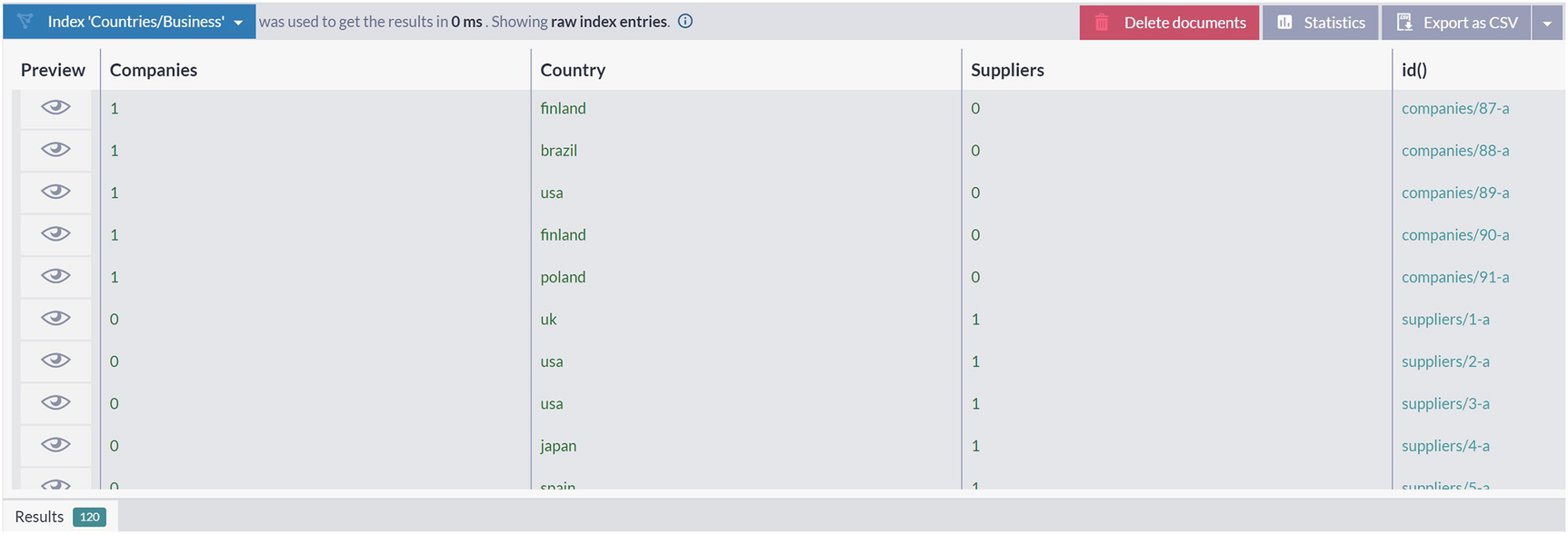
A snapshot of the company, suppliers, and country lists.

Figure 6-11

Raw Indexing Entries of MultiMap Index Countries/Business

As you can see, for every company and supplier document being processed, the index will extract its country, along with a count of one in an appropriate property.

All that is left to do now is to add aggregation. Hence, we expand the index with the reduction phase, which gives us the final form as shown in Listing 6-8 .
map("Companies", company => {
    return {
        Country: company.Address.Country,
        Companies: 1,
        Suppliers: 0
    }
})
map("Suppliers", company => {
    return {
        Country: company.Address.Country,
        Companies: 0,
        Suppliers: 1
    }
})
groupBy(map => map.Country)
    .aggregate(group => {
        return {
            Country: group.key,
            Companies: group.values.reduce((res, el) => res + el.Companies, 0),
            Suppliers: group.values.reduce((res, el) => res + el.Suppliers, 0)
        }
    })
Listing 6-8

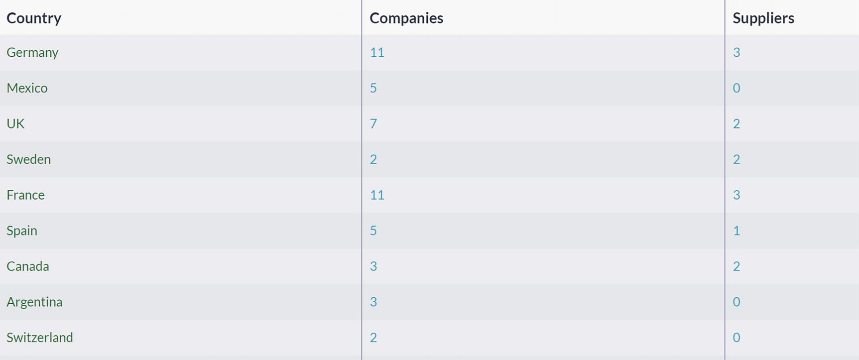
MultiMapReduce index Countries/Business

Finally, you can run the query:
from index 'Countries/Business'

to get a listing of countries with the number of companies and suppliers .

Artificial Documents

In addition to computing aggregations and storing them in an index, you can also materialize such indexing entries into documents called artificial documents. They will reside in a collection with an arbitrary name; every time the index is updated, this collection is also updated. This section will show scenarios when you want to create an artificial document, a walkthrough of their configuration, and to know how to perform indexing on them.

Querying index from Listing 6-8 will give raw indexing result as shown in Figure 6-12.

A snapshot of the country, company, and suppliers list.

Figure 6-12

Raw Indexing Entries of Countries/Business Index

You can now use these two fields of the index to order countries by the number of companies we do business with:
from index 'Countries/Business'
order by Companies as long desc
and by number of suppliers
from index 'Countries/Business'
order by Suppliers as long desc

However, what if we want to see totals? If you are making a business trip, which city would be your first choice? At which location would you have a chance to visit the most significant number of business entities your company is doing business with?

One way to solve this would be to expand index with additional field Total that would summarize Companies and Businesses, as shown in Listing 6-9.
map("Companies", company => {
    return {
        Country: company.Address.Country,
        Companies: 1,
        Suppliers: 0,
        Total: 1
    }
})
map("Suppliers", company => {
    return {
        Country: company.Address.Country,
        Companies: 0,
        Suppliers: 1,
        Total: 1
    }
})
groupBy(map => map.Country)
    .aggregate(group => {
        return {
            Country: group.key,
            Companies: group.values.reduce((res, el) => res + el.Companies, 0),
            Suppliers: group.values.reduce((res, el) => res + el.Suppliers, 0),
            Total: group.values.reduce((res, el) => res + el.Total, 0)
        }
    })
Listing 6-9

Countries/Business Index Expanded with Total

With an expanded index, you can now query:
from index 'Countries/Business'
order by Total as long desc

to get desired information.

Instead of expanding the index, you might want to go with a query shown in Listing 6-10.
from index 'Countries/Business'
order by (Companies + Suppliers) as long desc
Listing 6-10

Querying index with a computed field

Executing this query will result in an error.

In Chapter 4 , we talked about RavenDB’s approach to indexing – all of your queries are always executed against indexes, and precomputed index entries are used to provide blazingly fast responses from the database. Under no circumstances can queries contain any computation. All such calculations must be done within the index itself, ahead of query time. Precisely for this reason, a query from Listing 6-10 will result in an error – we attempted to sum up Companies and Suppliers and then order countries based on that criterion. Revisiting the expanded index from Listing 6-9, you can see that we are performing totals summing in the indexing phase indeed.

Inspecting raw indexing entries of the index before expansion, shown in Figure 6-12, reveals a data structure that would be appropriate for writing a simple map index. Unfortunately, RavenDB indexes can operate only on documents, not on raw indexing entries within other indexes.

However, RavenDB provides a way to materialize raw indexing entries into actual documents, so you can query or even index them. In the next section, we will show how to achieve this.

Creating Artificial Documents

Start by returning index Countries/Business to the state from Listing 6-8 before expanding it with field Total. When you open the index for editing, right below Reduce script area, there is an Output Reduce Results to Collection option, as shown in Figure 6-13.

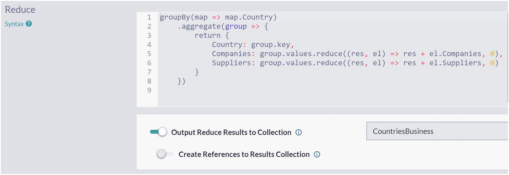
A snapshot of the company and supplier group value code.

Figure 6-13

Outputting Index Reduce Results to CountriesBusiness Artificial Collection

As a result, raw index entries, the same one you can see in Figure 6-12, will be extracted and loaded into proper JSON documents. If you check the list of collections, you will notice a new one there – CountriesBusiness – as shown in Figure 6-14.

A snapshot of the document id, company, supplier, and country list.

Figure 6-14

Documents in the Artificial Collection CountriesBusiness

This collection is called the artificial collection, and documents belonging to this collection are artificial documents. Opening one of these documents will reveal structure like one shown in Listing 6-11.
{
    "Country": "Finland",
    "Companies": 2,
    "Suppliers": 1,
    "@metadata": {
        "@collection": "CountriesBusiness",
        "@flags": "Artificial, FromIndex"
    }
}
Listing 6-11

Structure of one artificial document

Artificial documents can be created from MapReduce or MultiMapReduce indexes, containing indexing entries. If you compare raw indexing entries from Figure 6-12 with the content of the generated artificial collection, you will see that artificial collection represents a dump of an index. Artificial documents will contain all index fields as properties, and its metadata property will have a flag marking it as Artificial, FromIndex.

Every time a new order is created or an existing one is updated/deleted, all indexes indexing orders will be updated. The same thing will happen with the Countries/Business index, and its aggregated entries will be incrementally updated to take into account the latest changes. Additionally, since Countries/Business has output collection defined, this artificial collection will be updated.

Besides being automatically created by RavenDB, artificial documents are completely normal documents. Hence, you can run queries like
from 'CountriesBusiness'
where Country = 'UK'
to get number of companies and suppliers from the United Kingdom and
from 'CountriesBusiness'
where Companies > 1 and Suppliers > 1
select Country

to get a list of countries with at least one Company and Supplier .

Indexing Artificial Documents

After executing two queries from the previous section, you will discover that RavenDB created automatic index Auto/CountriesBusiness/ByCompaniesAndCountryAndSuppliers, which is expected behavior from your database.

Artificial documents are completely regular documents, so it is also possible to write Map or even MapReduce indexes which would process and aggregate them if needed. Hence to answer our original quest of finding countries with most suppliers and companies, we can first start by defining Map index CountriesBusiness/Totals, as shown in Listing 6-12.
map("CountriesBusiness", entry => {
    return {
        Country: entry.Country,
        Total: entry.Companies + entry.Suppliers
    }
})
Listing 6-12

CountriesBusiness/Totals index

You can now finally execute a query that will produce a list of countries, ordered by business activities in descending order :
from index 'CountriesBusiness/Totals'
order by Total as long desc
select Country

It is easy to see that your next business trip should be to the United States, Germany, and France.

Summary

This chapter introduced MapReduce and MultiMapReduce indexes to group and aggregate data. We introduced techniques for writing static versions of these indexes, along with a way to materialize their content into artificial documents. The next chapter will show how you can use RavenDB for full-text searching of your data.

..................Content has been hidden....................

You can't read the all page of ebook, please click here login for view all page.
Reset
18.220.127.68