
14
QUANTUM AND POST-QUANTUM

Previous chapters focused on cryptography today, but in this chapter I’ll examine the future of cryptography over a time horizon of, say, a century or more—one in which quantum computers exist. Quantum computers are computers that leverage phenomena from quantum physics in order to run different kinds of algorithms than the ones we’re used to. Quantum computers don’t exist yet and look very hard to build, but if they do exist one day, then they’ll have the potential to break RSA, Diffie–Hellman, and elliptic curve cryptography—that is, all the public-key crypto deployed or standardized as of this writing.
To insure against the risk posed by quantum computers, cryptography researchers have developed alternative public-key crypto algorithms called post-quantum algorithms that would resist quantum computers. In 2015, the NSA called for a transition to quantum-resistant algorithms designed to be safe even in the face of quantum computers, and in 2017 the US standardization agency NIST began a process that will eventually standardize post-quantum algorithms.
This chapter will thus give you a nontechnical overview of the principles behind quantum computers as well as a glimpse of post-quantum algorithms. There’s some math involved, but nothing more than basic arithmetic and linear algebra, so don’t be scared by the unusual notations.
How Quantum Computers Work
Quantum computing is a model of computing that uses quantum physics to compute differently and do things that classical computers can’t, such as breaking RSA and elliptic curve cryptography efficiently. But a quantum computer is not a super-fast normal computer. In fact, quantum computers can’t solve any problem that is too hard for a classical computer, such as brute force search or NP-complete problems.
Quantum computers are based on quantum mechanics, the branch of physics that studies the behavior of subatomic particles, which behave truly randomly. Unlike classical computers, which operate on bits that are either 0 or 1, quantum computers are based on quantum bits (or qubits), which can be both 0 and 1 simultaneously—a state of ambiguity called superposition. Physicists discovered that in this microscopic world, particles such as electrons and photons behave in a highly counterintuitive way: before you observe an electron, the electron is not at a definite location in space, but in several locations at the same time (that is, in a state of superposition). But once you observe it—an operation called measurement in quantum physics—then it stops at a fixed, random location and is no longer in superposition. This quantum magic is what enables the creation of qubits in a quantum computer.
But quantum computers only work because of a crazier phenomenon called entanglement: two particles can be connected (entangled) in a way that observing the value of one gives the value of the other, even if the two particles are widely separated (kilometers or even light-years away from each other). This behavior is illustrated by the Einstein–Podolsky–Rosen (EPR) paradox and is the reason why Albert Einstein initially dismissed quantum mechanics. (See https://plato.stanford.edu/entries/qt-epr/ for an in-depth explanation of why.)
To best explain how a quantum computer works, we should distinguish the actual quantum computer (the hardware, composed of quantum bits) from quantum algorithms (the software that runs on it, composed of quantum gates). The next two sections discuss these two notions.
Quantum Bits
Quantum bits (qubits), or groups thereof, are characterized with numbers called amplitudes, which are akin to probabilities but aren’t exactly probabilities. Whereas a probability is a number between 0 and 1, an amplitude is a complex number of the form a + b × i, or simply a + bi, where a and b are real numbers, and i is an imaginary unit. The number i is used to form imaginary numbers, which are of the form bi, with b a real number. When i is multiplied by a real number, we get another imaginary number, and when it is multiplied by itself it gives –1; that is i2 = –1.
Unlike real numbers, which can be seen as belonging to a line (see Figure 14-1), complex numbers can be seen as belonging to a plane (a space with two dimensions), as shown in Figure 14-2. Here, the x-axis in the figure corresponds to the a in a + bi, the y-axis corresponds to the b, and the dotted lines correspond to the real and imaginary part of each number. For example, the vertical dotted line going from the point 3 + 2i down to 3 is two units long (the 2 in the imaginary part 2i).
Figure 14-1: View of real numbers as points on an infinite straight line
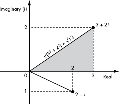
Figure 14-2: A view of complex numbers as points in a two-dimensional space
As you can see in Figure 14-2, you can use the Pythagorean theorem to compute the length of the line going from the origin (0) to the point a + bi by viewing this line as the diagonal of a triangle. The length of this diagonal is equal to the square root of the sum of the squared coordinates of the point, or √(a2 + b2), which we call the modulus of the complex number a + bi. We denote the modulus as |a + bi| and can use it as the length of a complex number.
In a quantum computer, registers consist of 1 or more qubits in a state of superposition characterized by a set of such complex numbers. But as we’ll see, these complex numbers—the amplitudes—can’t be any numbers.
Amplitudes of a Single Qubit
A single qubit is characterized by two amplitudes that I’ll call α (alpha) and β (beta). We can then express a qubit’s state as α |0〉 + β |1〉, where the “| 〉” notation is used to denote vectors in a quantum state. This notation then means that when you observe this qubit it will appear as 0 with a probability |α|2 and 1 with a probability |β|2. Of course, in order for these to be actual probabilities, |α|2 and |β|2 must be numbers between 0 and 1, and |α|2 + |β|2 must be equal to 1.
For example, say we have the qubit ![]() (psi) with amplitudes of α = 1/√2 and β = 1/√2. We can express this as follows:
(psi) with amplitudes of α = 1/√2 and β = 1/√2. We can express this as follows:
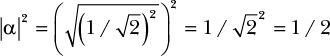
This notation means that in the qubit ![]() , the value 0 has an amplitude of 1/√2, and the value 1 has the same amplitude, 1/√2. To get the actual probability from the amplitudes, we compute the modulus of 1/√2 (which is equal to 1/√2, because it has no imaginary part), then square it: (1/√2)2 = 1/2. That is, if you observe the qubit
, the value 0 has an amplitude of 1/√2, and the value 1 has the same amplitude, 1/√2. To get the actual probability from the amplitudes, we compute the modulus of 1/√2 (which is equal to 1/√2, because it has no imaginary part), then square it: (1/√2)2 = 1/2. That is, if you observe the qubit ![]() , you’ll have a 1/2 chance of seeing a 0, and the same chance of seeing a 1.
, you’ll have a 1/2 chance of seeing a 0, and the same chance of seeing a 1.
Now consider the qubit Φ (phi), where
The qubit Φ is fundamentally distinct from ![]() because unlike
because unlike ![]() , where amplitudes have equal values, the qubit Φ has distinct amplitudes of α = i/√2 (a positive imaginary number) and β = –1/√2 (a negative real number). If, however, you observe Φ, the chance of your seeing a 0 or 1 is 1/2, the same as it is with
, where amplitudes have equal values, the qubit Φ has distinct amplitudes of α = i/√2 (a positive imaginary number) and β = –1/√2 (a negative real number). If, however, you observe Φ, the chance of your seeing a 0 or 1 is 1/2, the same as it is with ![]() . Indeed, we can compute the probability of seeing a 0 as follows, based on the preceding rules:
. Indeed, we can compute the probability of seeing a 0 as follows, based on the preceding rules:
NOTE
Because α = i/√2, α can be written as a + bi with a = 0 and b = 1/√2, and computing |α| = √(a2 + b2) yields 1/√2.
The upshot is that different qubits can behave similarly to an observer (with the same probability of seeing a 0 for both qubits) but have different amplitudes. This tells us that the actual probabilities of seeing a 0 or a 1 only partially characterize a qubit; just as when you observe the shadow of an object on a wall, the shape of the shadow will give you an idea of the object’s width and height, but not of its depth. In the case of qubits, this hidden dimension is the value of its amplitude: Is it positive or negative? Is it a real number or an imaginary number?
NOTE
To simplify notations, a qubit is often simply written as its pair of amplitudes (α, β). Our previous example can then be written |![]() 〉 = (1/√2, 1/√2).
〉 = (1/√2, 1/√2).
Amplitudes of Groups of Qubits
We’ve explored single qubits, but how do we understand multiple qubits? For example, a quantum byte can be formed with 8 qubits, when put into a state where the quantum states of these 8 qubits are somehow connected to each other (we say that the qubits are entangled, which is a complex physical phenomenon). Such a quantum byte can be described as follows, where the αs are the amplitudes associated with each of the 256 possible values of the group of 8 qubits:
Note that we must have |α0|2 + |α1|2 + . . . + |α255|2 = 1, so that all probabilities sum to 1.
Our group of 8 qubits can be viewed as a set of 28 = 256 amplitudes, because it has 256 possible configurations, each with its own amplitude. In physical reality, however, you’d only have eight physical objects, not 256. The 256 amplitudes are an implicit characteristic of the group of 8 qubits; each of these 256 numbers can take any of infinitely many different values. Generalizing, a group of n qubits is characterized by a set of 2n complex numbers, a number that grows exponentially with the numbers of qubits.
This encoding of exponentially many high-precision complex numbers is a core reason why a classical computer can’t simulate a quantum computer: in order to do so, it would need an unfathomably high amount of memory (of size around 2n) to store the same amount of information contained in only n qubits.
Quantum Gates
The concepts of amplitude and quantum gates are unique to quantum computing. Whereas a classical computer uses registers, memory, and a microprocessor to perform a sequence of instructions on data, a quantum computer transforms a group of qubits reversibly by applying a series of quantum gates, and then measures the value of one or more qubits. Quantum computers promise more computing power because with only n qubits, they can process 2n numbers (the qubits’ amplitudes). This property has profound implications.
From a mathematical standpoint, quantum algorithms are essentially a circuit of quantum gates that transforms a set of complex numbers (the amplitudes) before a final measurement where the value of 1 or more qubits is observed (see Figure 14-3). You’ll also see quantum algorithms referred to as quantum gate arrays or quantum circuits.
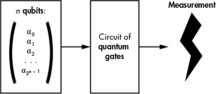
Figure 14-3: Principle of a quantum algorithm
Quantum Gates as Matrix Multiplications
Unlike the Boolean gates of a classical computer (AND, XOR, and so on), a quantum gate acts on a group of amplitudes just as a matrix acts when multiplied with a vector. For example, in order to apply the simplest quantum gate, the identity gate, to the qubit Φ, we see I as a 2 × 2 matrix and multiply it with the column vector consisting of the two amplitudes of Φ, as shown here:
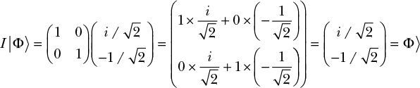
The result of this matrix–vector multiplication is another column vector with two elements, where the top value is equal to the dot product of the I matrix’s first line with the input vector (the result of adding the product of the first elements 1 and i/√2 to the product of the second elements 0 and –1/√2), and likewise for the bottom value.
NOTE
In practice, a quantum computer wouldn’t explicitly compute matrix–vector multiplications because the matrices would be way too large. (That’s why quantum computing can’t be simulated by a classical computer.) Instead, a quantum computer would transform qubits as physical particles through physical transformations that are equivalent to a matrix multiplication. Confused? Here’s what Richard Feynman had to say: “If you are not completely confused by quantum mechanics, you do not understand it.”
The Hadamard Quantum Gate
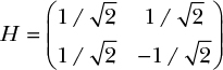
The only quantum gate we’ve seen so far, the identity gate I, is pretty useless because it doesn’t do anything and leaves a qubit unchanged. Now we’re going to see one of the most useful quantum gates, called the Hadamard gate, usually denoted H. The Hadamard gate is defined as follows (note the negative value in the bottom-right position):
Let’s see what happens if we apply this gate to the qubit |![]() 〉 = (1/√2, 1/√2):
〉 = (1/√2, 1/√2):
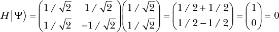
By applying the Hadamard gate H to |![]() 〉, we obtain the qubit |0〉 for which the value |0〉 has amplitude 1, and |1〉 has amplitude 0. This tells us that the qubit will behave deterministically: that is, if you observe this qubit, you would always see a 0 and never a 1. In other words, we’ve lost the randomness of the initial qubit |
〉, we obtain the qubit |0〉 for which the value |0〉 has amplitude 1, and |1〉 has amplitude 0. This tells us that the qubit will behave deterministically: that is, if you observe this qubit, you would always see a 0 and never a 1. In other words, we’ve lost the randomness of the initial qubit |![]() 〉.
〉.
What happens if we apply the Hadamard gate again to the qubit |0〉?
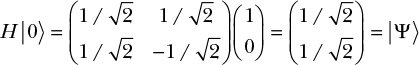
This brings us back to the qubit |![]() 〉 and a randomized state. Indeed, the Hadamard gate is often used in quantum algorithms to go from a deterministic state to a uniformly random one.
〉 and a randomized state. Indeed, the Hadamard gate is often used in quantum algorithms to go from a deterministic state to a uniformly random one.
Not All Matrices are Quantum Gates
Although quantum gates can be seen as matrix multiplications, not all matrices correspond to quantum gates. Recall that a qubit consists of the complex numbers α and β and the amplitudes of the qubit, such that they satisfy the condition |α|2 + |β|2 = 1. If after multiplying a qubit by a matrix we get two amplitudes that don’t match this condition, the result can’t be a qubit. Quantum gates can only correspond to matrices that preserve the property |α|2 + |β|2 = 1, and matrices that satisfy this condition are called unitary matrices.
Unitary matrices (and quantum gates by definition) are invertible, meaning that given the result of an operation, you can compute back the original qubit by applying the inverse matrix. This is the reason why quantum computing is said to be a kind of reversible computing.
Quantum Speed-Up
A quantum speed-up occurs when a problem can be solved faster by a quantum computer than by a classical one. For example, in order to search for an item among n items of an unordered list on a classical computer, you need on average n/2 operations, because you need to look at each item in the list before finding the one you’re looking for. (On average, you’ll find that item after searching half of the list.) No classical algorithm can do better than n/2. However, a quantum algorithm exists to search for an item in only about √n operations, which is orders of magnitude smaller than n/2. For example, if n is equal to 1000000, then n/2 is 500000, whereas √n is 1000.
We attempt to quantify the difference between quantum and classical algorithms in terms of time complexity, which is represented by O() notation. In the previous example, the quantum algorithm runs in time O(√n) but the classical algorithm can’t be faster than O(n). Because the difference in time complexity here is due to the square exponent, we call this quadratic speed-up. But while such a speed-up will likely make a difference, there are much more powerful ones.
Exponential Speed-Up and Simon’s Problem
Exponential speed-ups are the Holy Grail of quantum computing. They occur when a task that takes an exponential amount of time on a classical computer, such as O(2n), can be performed on a quantum computer with polynomial complexity—namely O(nk) for some fixed number k. This exponential speed-up can turn a practically impossible task into a possible one. (Recall from Chapter 9 that cryptographers and complexity theorists associate exponential time with the impossible, and they associate polynomial time with the practical.)
The poster child of exponential speed-ups is Simon’s problem. In this computational problem, a function, f(), transforms n-bit strings to n-bit strings, such that the output of f() looks random except that there is a value, m, such that any two values x, y that satisfies f(x) = f(y), then y = x ⊕ m. The way to solve this problem is to find m.
The route to take when solving Simon’s problem with a classical algorithm boils down to finding a collision, which takes approximately 2n/2 queries to f(). However, a quantum algorithm (shown in Figure 14-4) can solve Simon’s problem in approximately n queries, with the extremely efficient time complexity of O(n).
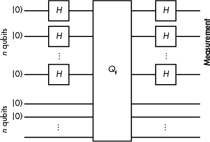
Figure 14-4: The circuit of the quantum algorithm that solves Simon’s problem efficiently
As you can see in Figure 14-4, you initialize 2n qubits to |0〉, apply Hadamard gates (H) to the first n qubits, then apply the gate Qf to the two groups of all n qubits. Given two n-qubit groups x and y, the gate Qf transforms the quantum state |x〉|y〉 to the state |x〉|f(x) ⊕ y〉. That is, it computes the function f() on the quantum state reversibly, because you can go from the new state to the old one by computing f(x) and XORing it to f(x) ⊕ y. (Unfortunately, explaining why all of this works is beyond the scope of this book.)
The exponential speed-up for Simon’s problem can be used against symmetric ciphers only in very specific cases, but in the next section you’ll see some real crypto-killer applications of quantum computing.
The Threat of Shor’s Algorithm
In 1995, AT&T researcher Peter Shor published an eye-opening article titled “Polynomial-Time Algorithms for Prime Factorization and Discrete Logarithms on a Quantum Computer.” Shor’s algorithm is a quantum algorithm that causes an exponential speed-up when solving the factoring, discrete logarithm (DLP), and elliptic curve discrete logarithm (ECDLP) problems. You can’t solve these problems with a classical computer, but you could with a quantum computer. That means that you could use a quantum computer to solve any cryptographic algorithm that relies on those problems, including RSA, Diffie–Hellman, elliptic curve cryptography, and all currently deployed public-key cryptography mechanisms. In other words, you could reduce the security of RSA or elliptic curve cryptography to that of Caesar’s cipher. (Shor might as well have titled his article “Breaking All Public-Key Crypto on a Quantum Computer.”) Shor’s algorithm has been called “one of the major scientific achievements of the late 20th century” by renowned complexity theorist Scott Aaronson.
Shor’s algorithm actually solves a more general class of problems than factoring and discrete logarithms. Specifically, if a function f() is periodic—that is, if there’s a ω (the period) such that f(x + ω) = f(x) for any x, Shor’s algorithm will efficiently find ω. (This looks very similar to Simon’s problem discussed previously, and indeed Simon’s algorithm was a major inspiration for Shor’s algorithm.) The ability of Shor’s algorithm to efficiently compute the period of a function is important to cryptographers because that ability can be used to attack public-key cryptography, as I’ll discuss next.
A discussion of the details of how Shor’s algorithm achieves its speed-up is far too technical for this book, but in this section I’ll show how you could use Shor’s algorithm to attack public-key cryptography. Let’s see how Shor’s algorithm could be used to solve the factoring and discrete logarithm problems (as discussed in Chapter 9), which are respectively the hard problems behind RSA and Diffie–Hellman.
Shor’s Algorithm Solves the Factoring Problem
Say you want to factor a large number, N = pq. It’s easy to factor N if you can compute the period of ax mod N, a task that is hard to do with a classical computer but easy to do on a quantum one. You first pick a random number a less than N, and ask Shor’s algorithm to find the period ω of the function f(x) = ax mod N. Once you’ve found the period, you’ll have ax mod N = ax + ω mod N (that is, ax mod N = axaω mod N), which means that aω mod N = 1, or aω – 1 mod N = 0. In other words, aω – 1 is a multiple of N, or aω – 1 = kN for some unknown number k.
The key observation here is that you can easily factor the number aω – 1 as the product of two terms, where aω – 1 = (aω / 2 – 1)(aω / 2 + 1). You can then compute the greatest common divisor (GCD) between (aω / 2 – 1) and N, and check to see if you’ve obtained a nontrivial factor of N (that is, a value other than 1 or N). If not, you can just rerun the same algorithm with another value of a. After a few trials, you’ll get a factor of N. You’ve now recovered the private RSA key from its public key, which allows you to decrypt messages or forge signatures.
But just how easy is this computation? Note that the best classical algorithm to use to factor a number N runs in time exponential in n, the bit length of N (that is, n = log2 N). However, Shor’s algorithm runs in time polynomial in n—namely, O(n2(log n)(log log n)). This means that if we had a quantum computer, we could run Shor’s algorithm and see the result within a reasonable amount of time (days? weeks? months, maybe?) instead of thousands of years.
Shor’s Algorithm and the Discrete Logarithm Problem
The challenge in the discrete logarithm problem is to find y, given y = gx mod p, for some known numbers g and p. Solving this problem takes an exponential amount of time on a classical computer, but Shor’s algorithm lets you find y easily thanks to its efficient period-finding technique.
For example, consider the function f(a, b) = gayb. Say we want to find the period of this function, the numbers ω and ω′, such that f(a + ω, b + ω′) = f(a, b) for any a and b. The solution we seek is then x = –ω / ω′ modulo q, the order of g, which is a known parameter. The equality f(a + ω, b + ω′) = f(a, b) implies gωyω′ mod p = 1. By substituting y with gx, we have gω + xω′ mod p = 1, which is equivalent to ω + xω′ mod q = 0, from which we derive x = – ω / ω′.
Again, the overall complexity is O(n2(log n)(log log n)), with n the bit length of p. This algorithm generalizes to find discrete logarithms in any commutative group, not just the group of numbers modulo a prime number.
Grover’s Algorithm
After Shor’s algorithm exponential speed-up for factoring, another important form of quantum speed-up is the ability to search among n items in time proportional to the square root of n, whereas any classical algorithm would take time proportional to n. This quadratic speed-up is possible thanks to Grover’s algorithm, a quantum algorithm discovered in 1996 (after Shor’s algorithm). I won’t cover the internals of Grover’s algorithm because they’re essentially a bunch of Hadamard gates, but I’ll explain what kind of problem Grover solves and its potential impact on cryptographic security. I’ll also show why you can salvage a symmetric crypto algorithm from quantum computers by doubling the key or hash value size, whereas asymmetric algorithms are destroyed for good.
Think of Grover’s algorithm as a way to find the value x among n possible values, such that f(x) = 1, and where f(x) = 0 for most other values. If m values of x satisfy f(x) = 1, Grover will find a solution in time O(√(n / m)); that is, in time proportional to the square root of n divided by m. In comparison, a classical algorithm can’t do better than O(n / m).
Now consider the fact that f() can be any function. It could be, for example, “f(x) = 1 if and only if x is equal to the unknown secret key K such that E(K, P) = C” for some known plaintext P and ciphertext C, and where E() is some encryption function. In practice, this means that if you’re looking for a 128-bit AES key with a quantum computer, you’ll find the key in time proportional to 264, rather than 2128 if you had only classical computers. You would need a large enough plaintext to ensure the uniqueness of the key. (If the plaintext and ciphertext are, say, 32 bits, many candidate keys would map that plaintext to that ciphertext.) The complexity 264 is much smaller than 2128, meaning that a secret key would be much easier to recover. But there’s an easy solution: to restore 128-bit security, just use 256-bit keys! Grover’s algorithm will then reduce the complexity of searching a key to “only” 2256 / 2 = 2128 operations.
Grover’s algorithm can also find preimages of hash functions (a notion discussed in Chapter 6). To find a preimage of some value h, the f() function is defined as “f(x) = 1 if and only if Hash(x) = h, otherwise f(x) = 0.” Grover thus gets you preimages of n-bit hashes at the cost of the order of 2n/2 operations. As with encryption, to ensure 2n post-quantum security, just use hash values twice as large, since Grover’s algorithm will find a preimage of a 2n-bit value in at least 2n operations.
The bottom line is that you can salvage symmetric crypto algorithms from quantum computers by doubling the key or hash value size, whereas asymmetric algorithms are destroyed for good.
NOTE
There is a quantum algorithm that finds hash function collisions in time O(2n/3), instead of O(2n/2), as with the classic birthday attack. This would suggest that quantum computers can outperform classical computers for finding hash function collisions, except that the O(2n/3)-time quantum algorithm also requires O(2n/3) space, or memory, in order to run. Give O(2n/3) worth of computer space to a classic algorithm and it can run a parallel collision search algorithm with a collision time of only O(2n/6), which is much faster than the O(2n/3) quantum algorithm. (For details of this attack, see “Cost Analysis of Hash Collisions” by Daniel J. Bernstein at http://cr.yp.to/papers.html#collisioncost.)
Why Is It So Hard to Build a Quantum Computer?
Although quantum computers can in principle be built, we don’t know how hard it will be or when that might happen, if at all. And so far, it looks really hard. As of early 2017, the record holder is a machine that is able to keep 14 (fourteen!) qubits stable for only a few milliseconds, whereas we’d need to keep millions of qubits stable for weeks in order to break any crypto. The point is, we’re not there yet.
Why is it so hard to build a quantum computer? Because you need extremely small things to play the role of qubits—about the size of electrons or photons. And because qubits must be so small, they’re also extremely fragile.
Qubits must also be kept at extremely low temperatures (close to absolute zero) in order to remain stable. But even at such a freezing temperature, the state of the qubits decays, and they eventually become useless. As of this writing, we don’t yet know how to make qubits that will last for more than a couple of seconds.
Another challenge is that qubits can be affected by the environment, such as heat and magnetic fields, which can create noise in the system, and hence computation errors. In theory, it’s possible to deal with these errors (as long as the error rate isn’t too high), but it’s hard to do so. Correcting qubits’ errors requires specific techniques called quantum error-correcting codes, which in turn require additional qubits and a low enough rate of error. But we don’t know how to build systems with such a low error rate.
At the moment, there are two main approaches to forming qubits, and therefore to building quantum computers: superconducting circuits and ion traps. Using superconducting circuits is the approach championed by labs at Google and IBM. It’s based on forming qubits as tiny electrical circuits that rely on quantum phenomena from superconductor materials, where charge carriers are pairs of electrons. Qubits made of superconducting circuits need to be kept at temperatures close to absolute zero, and they have a very short lifetime. The record as of this writing is nine qubits kept stable for a few microseconds.
Ion traps, or trapped ions, are made up of ions (charged atoms) and are manipulated using lasers in order to prepare the qubits in specific initial states. Using ion traps was one of the first approaches to building qubits, and they tend to be more stable than superconducting circuits. The record as of this writing is 14 qubits stable for a few milliseconds. But ion traps are slower to operate and seem harder to scale than superconducting circuits.
Building a quantum computer is really a moonshot effort. The challenge comes down to 1) building a system with a handful of qubits that is stable, fault tolerant, and capable of applying basic quantum gates, and 2) scaling such a system to thousands or millions of qubits to make it useful. From a purely physical standpoint, and to the best of our knowledge, there is nothing to prevent the creation of large fault-tolerant quantum computers. But many things are possible in theory and prove hard or too costly to realize in practice (like secure computers). Of course, the future will tell who is right—the quantum optimists (who sometimes predict a large quantum computer in ten years) or the quantum skeptics (who argue that the human race will never see a quantum computer).
Post-Quantum Cryptographic Algorithms
The field of post-quantum cryptography is about designing public-key algorithms that cannot be broken by a quantum computer; that is, they would be quantum safe and able to replace RSA and elliptic curve–based algorithms in a future where off-the-shelf quantum computers could break 4096-bit RSA moduli in a snap.
Such algorithms should not rely on a hard problem known to be efficiently solvable by Shor’s algorithm, which kills the hardness in factoring and discrete logarithm problems. Symmetric algorithms such as block ciphers and hash functions would lose only half their theoretical security in the face of a quantum computer but would not be badly broken as RSA. They might constitute the basis for a post-quantum scheme.
In the following sections, I explain the four main types of post-quantum algorithms: code-based, lattice-based, multivariate, and hash-based. Of these, hash-based is my favorite because of its simplicity and strong security guarantees.
Code-Based Cryptography
Code-based post-quantum cryptographic algorithms are based on error-correcting codes, which are techniques designed to transmit bits over a noisy channel. The basic theory of error-correcting codes dates back to the 1950s. The first code-based encryption scheme (the McEliece cryptosystem) was developed in 1978 and is still unbroken. Code-based crypto schemes can be used for both encryption and signatures. Their main limitation is the size of their public key, which is typically on the order of a hundred kilobytes. But is that really a problem when the average size of a web page is around two megabytes?
Let me first explain what error-correcting codes are. Say you want to transmit a sequence of bits as a sequence of (say) 3-bit words, but the transmission is unreliable and you’re concerned that 1 or more bits may be incorrectly transmitted: you send 010, but the receiver gets 011. One simple way to address this would be to use a very basic error-correction code: instead of transmitting 010 you would transmit 000111000 (repeating each bit three times), and the receiver would decode the received word by taking the majority value for each of the three bits. For example, 100110111 would be decoded to 011 because that pattern appears twice. But as you can see, this particular error-correcting code would allow a receiver to correct only up to one error per 3-bit chunk, because if two errors occur in the same 3-bit chunk, the majority value would be the wrong one.
Linear codes are an example of less trivial error-correcting codes. In the case of linear codes, a word to encode is seen as an n-bit vector v, and encoding consists of multiplying v with an m × n matrix G to compute the code word w = vG. (In this example, m is greater than n, meaning that the code word is longer than the original word.) The value G can be structured such that for a given number t, any t-bit error in w allows the recipient to recover the correct v. In other words, t is the maximum number of errors that can be corrected.
In order to encrypt data using linear codes, the McEliece cryptosystem constructs G as a secret combination of three matrices, and encrypts by computing w = vG plus some random value, e, which is a fixed number of 1 bit. Here, G is the public key, and the private key is composed of the matrices A, B, and C such that G = ABC. Knowing A, B, and C allows one to decode a message reliably and retrieve w. (You’ll find the decoding step described online.)
The security of the McEliece encryption scheme relies on the hardness of decoding a linear code with insufficient information, a problem known to be NP-complete and therefore out of reach of quantum computers.
Lattice-Based Cryptography
Lattices are mathematical structures that essentially consist of a set of points in an n-dimensional space, with some periodic structure. For example, in dimension two (n = 2), a lattice can be viewed as the set of points shown in Figure 14-5.
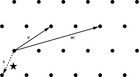
Figure 14-5: Points of a two-dimensional lattice, where v and w are basis vectors of the lattice, and s is the closest vector to the star-shaped point
Lattice theory has led to deceptively simple cryptography schemes. I’ll give you the gist of it.
A first hard problem found in lattice-based crypto is known as short integer solution (SIS). SIS consists of finding the secret vector s of n numbers given (A, b) such that b = As mod q, where A is a random m × n matrix and q is a prime number.
The second hard problem in lattice-based cryptography is called learning with errors (LWE). LWE consists of finding the secret vector s of n numbers given (A, b), where b = As + e mod q, with A being a random m × n matrix, e a random vector of noise, and q a prime number. This problem looks a lot like noisy decoding in code-based cryptography.
SIS and LWE are somewhat equivalent, and can be restated as instances of the closest vector problem (CVP) on a lattice, or the problem of finding the vector in a lattice closest to a given point, by combining a set of basis vectors. The dotted vector s in Figure 14-5 shows how we would find the closest vector to the star-shaped point by combining the basis vectors v and w.
CVP and other lattice problems are believed to be hard both for classical and quantum computers. But this doesn’t directly transfer to secure cryptosystems, because some problems are only hard in the worst case (that is, for their hardest instance) rather than the average case (which is what we need for crypto). Furthermore, while finding the exact solution to CVP is hard, finding an approximation of the solution can be considerably easier.
Multivariate Cryptography
Multivariate cryptography is about building cryptographic schemes that are as hard to break as it is to solve systems of multivariate equations, or equations involving multiple unknowns. Consider, for example, the following system of equations involving four unknowns x1, x2, x3, x4:
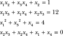
These equations consist of the sum of terms that are either a single unknown, such as x4 (or terms of degree one), or the product of two unknown values, such as x2x3 (terms of degree two or quadratic terms). To solve this system, we need to find the values of x1, x2, x3, x4 that satisfy all four equations. Equations may be over all real numbers, integers only, or over finite sets of numbers. In cryptography, however, equations are typically over numbers modulo some prime numbers, or over binary values (0 and 1).
The problem here is to find a solution that is NP-hard given a random quadratic system of equations. This hard problem, known as multivariate quadratics (MQ) equations, is therefore a potential basis for post-quantum systems because quantum computers won’t solve NP-hard problems efficiently.
Unfortunately, building a cryptosystem on top on MQ isn’t so straightforward. For example, if we were to use MQ for signatures, the private key might consist of three systems of equations, L1, N, and L2, which when combined in this order would give another system of equations that we’ll call P, the public key. Applying the transformations L1, N, and L2 consecutively (that is, transforming a group of values as per the system of equations) is then equivalent to applying P by transforming x1, x2, x3, x4 to y1, y2, y3, y4, defined as follows:
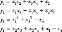
In such a cryptosystem, L1, N, and L2 are chosen such that L1 and L2 are linear transformations (that is, having equations where terms are only added, not multiplied) that are invertible, and where N is a quadratic system of equations that is also invertible. This makes the combination of the three a quadratic system that’s also invertible, but whose inverse is hard to determine without knowing the inverses of L1, N, and L2.
Computing a signature then consists of computing the inverses of L1, N, and L2 applied to some message, M, seen as a sequence of variables, x1, x2, . . . .
S = L2−1(N−1(L1−(M)))
Verifying a signature then consists of verifying that P(S) = M.
Attackers could break such a cryptosystem if they manage to compute the inverse of P, or to determine L1, N, and L2 from P. The actual hardness of solving such problems depends on the parameters of the scheme, such as the number of equations used, the size and type of the numbers, and so on. But choosing secure parameters is hard, and more than one multivariate scheme considered safe has been broken.
Multivariate cryptography isn’t used in major applications due to concerns about the scheme’s security and because it’s often slow or requires tons of memory. A practical benefit of multivariate signature schemes, however, is that it produces short signatures.
Hash-Based Cryptography
Unlike the previous schemes, hash-based cryptography is based on the well-established security of cryptographic hash functions rather than on the hardness of mathematical problems. Because quantum computers cannot break hash functions, they cannot break anything that relies on the difficulty of finding collisions, which is the key idea of hash function–based signature schemes.
Hash-based cryptographic schemes are pretty complex, so we’ll just take a look at their simplest building block: the one-time signature, a trick discovered around 1979, and known as Winternitz one-time signature (WOTS), after its inventor. Here “one-time” means that a private key can be used to sign only one message; otherwise, the signature scheme becomes insecure. (WOTS can be combined with other methods to sign multiple messages, as you’ll see in the subsequent section.)
But first, let’s see how WOTS works. Say you want to sign a message viewed as a number between 0 and w – 1, where w is some parameter of the scheme. The private key is a random string, K. To sign a message, M, with 0 ≤ M < w, you compute Hash(Hash(. . .(Hash(K))), where the hash function Hash is repeated M times. We denote this value as HashM(K). The public key is Hashw(K), or the result of w nested iterations of Hash, starting from K.
A WOTS signature, S, is verified by checking that Hashw – M(S) is equal to the public key Hashw(K). Note that S is K after M applications of Hash, so if we do another w – M applications of Hash, we’ll get a value equal to K hashed M + (w – M) = w times, which is the public key.
This scheme looks rather dumb, and it has significant limitations:
Signatures can be forged
From HashM(K), the signature of M, you can compute Hash(HashM(K)) = HashM + 1(K), which is a valid signature of the message M + 1. This problem can be fixed by signing not only M, but also w – M, using a second key.
It only works for short messages
If messages are 8 bits long, there are up to 28 – 1 = 255 possible messages, so you’ll have to compute Hash up to 255 times in order to create a signature. That might work for short messages, but not for longer ones: for example, with 128-bit messages, signing the message 2128 – 1 would take forever. A workaround is to split longer messages into shorter ones.
It works only once
If a private key is used to sign more than one message, an attacker can recover enough information to forge a signature. For example, if w = 8 and you sign the numbers 1 and 7 using the preceding trick to avoid trivial forgeries, the attacker gets Hash1(K) and Hash7(K′) as a signature of 1, and Hash7(K) and Hash1(K′) as a signature of 7. From these values, the attacker can compute Hashx(K) and Hashx(K′) for any x in [1;7] and thus forge a signature on behalf of the owner of K and K′. There is no simple way to fix this.
State-of-the-art hash-based schemes rely on more complex versions of WOTS, combined with tree data structures and sophisticated techniques designed to sign different messages with different keys. Unfortunately, the resulting schemes produce large signatures (on the order of dozens of kilobytes, as with SPHINCS, a state-of-the-art scheme at the time of this writing), and they sometimes have a limit on the number of messages they can sign.
How Things Can Go Wrong
Post-quantum cryptography may be fundamentally stronger than RSA or elliptic curve cryptography, but it’s not infallible or omnipotent. Our understanding of the security of post-quantum schemes and their implementations is more limited than for not-post-quantum cryptography, which brings with it increased risk, as summarized in the following sections.
Unclear Security Level
Post-quantum schemes can appear deceptively strong yet prove insecure against both quantum and classical attacks. Lattice-based algorithms, such as the ring-LWE family of computational problems (versions of the LWE problem that work with polynomials), are sometimes problematic. Ring-LWE is attractive for cryptographers because it can be leveraged to build cryptosystems that are in principle as hard to break as it is to solve the hardest instances of Ring-LWE problems, which can be NP-hard. But when security looks too good to be true, it often is.
One problem with security proofs is that they are often asymptotic, meaning that they’re true only for a large number of parameters such as the dimension of the underlying lattice. However, in practice, a much smaller number of parameters is used.
Even when a lattice-based scheme looks to be as hard to break as some NP-hard problem, its security remains hard to quantify. In the case of lattice-based algorithms, we rarely have a clear picture of the best attacks against them and the cost of such an attack in terms of computation or hardware, because of our lack of understanding of these recent constructions. This uncertainty makes lattice-based schemes harder to compare against better-understood constructions such as RSA, and this scares potential users. However, researchers have been making progress on this front and hopefully in a few years, lattice problems will be as well understood as RSA. (For more technical details on the Ring-LWE problem, read Peikert’s excellent survey at https://eprint.iacr.org/2016/351/.)
Fast Forward: What Happens if It’s Too Late?
Imagine this CNN headline: April 2, 2048: “ACME, Inc. reveals its secretly built quantum computer, launches break-crypto-as-a-service platform.” Okay, RSA and elliptic curve crypto are screwed. Now what?
The bottom line is that post-quantum encryption is way more critical than post-quantum signatures. Let’s look at the case of signatures first. If you were still using RSA-PSS or ECDSA as a signature scheme, you could just issue new signatures using a post-quantum signature scheme in order to restore your signatures’ trust. You would revoke your older, quantum-unsafe public keys and compute fresh signatures for every message you had signed. After a bit of work, you’d be fine.
You would only need to panic if you were encrypting data using quantum-
unsafe schemes, such as RSA-OAEP. In this case all transmitted ciphertext could be compromised. Obviously, it would be pointless to encrypt that plaintext again with a post-quantum algorithm since your data’s confidentiality is already gone.
But what about key agreement, with Diffie–Hellman (DH) and its elliptic curve counterpart (ECDH)?
Well, at first glance, the situation looks to be as bad as with encryption: attackers who’ve collected public keys ga and gb could use their shiny new quantum computer to compute the secret exponent a or b and compute the shared secret gab, and then derive from it the keys used to encrypt your traffic. But in practice, Diffie–Hellman isn’t always used in such a simplistic fashion. The actual session keys used to encrypt your data may be derived from both the Diffie–Hellman shared secret and some internal state of your system.
For example, that’s how state-of-the-art mobile messaging systems work, thanks to a protocol pioneered with the Signal application. When you send a new message to a peer with Signal, a new Diffie–Hellman shared secret is computed and combined with some internal secrets that depend on the previous messages sent within that session (which can span long periods of time). Such advanced use of Diffie–Hellman makes the work of an attacker much harder, even one with a quantum computer.
Implementation Issues
In practice, post-quantum schemes will be code, not algorithms; that is, software running on some physical processor. And however strong the algorithms may be on paper, they won’t be immune to implementation errors, software bugs, or side-channel attacks. An algorithm may be completely post-quantum in theory but may still be broken by a simple classical computer program because a programmer forgot to enter a semicolon.
Furthermore, schemes such as code-based and lattice-based algorithms rely heavily on mathematical operations, the implementation of which uses a variety of tricks to make those operations as fast as possible. But by the same token, the complexity of the code in these algorithms makes implementation more vulnerable to side-channel attacks, such as timing attacks, which infer information about secret values based on measurement of execution times. In fact, such attacks have already been applied to code-based encryption (see https://eprint.iacr.org/2010/479/) and to lattice-based signature schemes (see https://eprint.iacr.org/2016/300/).
The upshot is that, ironically, post-quantum schemes will be less secure in practice at first than non-post-quantum ones, due to vulnerabilities in their implementations.
Further Reading
To learn the basics of quantum computation, read the classic Quantum Computation and Quantum Information by Nielsen and Chuang (Cambridge, 2000). Aaronson’s Quantum Computing Since Democritus (Cambridge, 2013), a less technical and more entertaining read, covers more than quantum computing.
Several software simulators will allow you to experiment with quantum computing. The Quantum Computing Playground at http://www.quantumplayground.net/ is particularly well designed, with a simple programming language and intuitive visualizations.
For the latest research in post-quantum cryptography, see https://pqcrypto.org/ and the associated conference PQCrypto.
The coming years promise to be particularly exciting for post-quantum crypto thanks to NIST’s Post-Quantum Crypto Project, a community effort to develop the future post-quantum standard. Be sure to check the project’s website http://csrc.nist.gov/groups/ST/post-quantum-crypto/ for the related algorithms, research papers, and workshops.