
Definitions and Some Concepts
Sometimes it is possible to represent random variables as a function in a way that the function can determine the probability of an outcome of the random variable.
Definition 4.1
The outcome of a random variable is determined by chance. The outcome of a random variable might be constant as in the case of observing a head when a coin is flipped, or it can be a variable value such as the length of time it takes for different students to learn this chapter. The subject “statistics” is used to study the properties of random variables and how they behave.
Definition 4.2
The probability distribution determines the probability of the outcomes of a random variable. In its simplest form, the probability distribution consists of values and probabilities. The probability distribution for flipping a coin is:
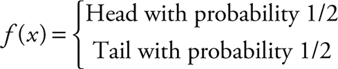
There are more formal ways to define probability distribution that are beyond the scope of this text. A distribution function can be presented in the form of a function, a table, or a statement. The subject of probability distribution is vast, but we will focus on the few items needed to continue our discussion. There are two types of random variables, discrete and continuous.
Definition 4.3
A discrete random variable consists of integers only.
Definition 4.4
A continuous random variable can take any value over a range.
Definition 4.5
The probability distribution for a discrete random variable is called a discrete probability distribution and is represented as f (x).
Definition 4.6
The probability distribution for a continuous random variable is called a probability density function.
In this text we may use distribution function for both discrete and continuous random variable as a matter of convenience.
Continuous Distribution Functions
There are numerous distribution functions, both discrete and continuous. In this text, for the sake of space only, the distribution functions that are used to provide inference are discussed.
Normal Distribution Function
Normal distribution functions are the most important and most widely used distribution function. Standardized normal distribution functions, called standard normal, can be applied in any area and situation, provided that one is assured of the normality and either knows, or can estimate, the mean and variance of the distribution. Standard normal values are the Z scores of values that have a normal distribution. Converting values from different normal distributions with different means and variances to standard normal allows us to compare them. Furthermore, any standardized value can be compared with the theoretical standard normal table.
Since normal distribution is a continuous distribution function, and there are infinitely many points on any continuous interval, the probability of any single point is always zero. For continuous distribution functions, such as normal distribution, the probability is calculated for an interval. Direct computation of such probabilities requires integral calculus. For simplicity, a table of standard normal values is used. Spreadsheets such as Microsoft Excel are capable of computing the standard normal values. A table of values for normal distribution is provided in the Appendix.
Properties of Normal Distribution
A normal distribution is depicted in Figure 4.1. The normal distribution curve is unimodal and symmetric. Consequently, its mean, mode, and median are all the same and fall in the middle of the curve. You may notice that the tails of the normal curve do not touch the x-axis. This is another property of the normal distribution. The x-axis is actually an asymptote of the functions, which means the curve does not touch the axis even at infinity. This implies that the tails are stretched to infinity, but in practice, we do not stretch the tails that far. As you will soon see, the probability of the tail areas becomes very negligible not too far from the center, making it unnecessary to be concerned with infinity. A normal distribution has two parameters: its mean and variance. In other words, the mean and variance of a normal distribution determine its specific center and spread. Since distribution is commonly used and has so many applications, it has become known as normal distribution. Furthermore, the mean and variance of the normal distribution are represented by μ and σ 2, respectively.
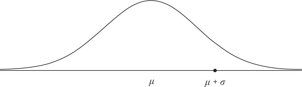
Figure 4.1. Normal distribution with mean = μ and variance = σ2.
The area under the normal curve is equal to 1, as is the area under any distribution density function. Customarily, the distance from the center of normal distribution is measured by its standard deviation. If two normal distribution functions have the same mean and variance then the area under the curve for two points that are the same distance from the center are equal. By converting any normal distribution to one with a mean of 0 and a standard deviation of 1, we are able to calculate the area under the curve between the center and any point for any normal distribution regardless of its mean and variance. The area under normal distribution represents the probability between any two points on the curve. We will soon see that the probability for a point to be within one standard deviation from the mean of a normal distribution function is about 68%. Since the normal distribution is symmetric, it is possible to calculate area from the center to a point on one side of the center, and the probability for a point of the same distance from the mean on the other side, which will be equal.
Standardizing Values from a Normal Distribution
In Chapter 3 we discussed Z score, which can be used to compare dissimilar things by converting them to the same basis, which is by obtaining their deviations from their expected values and scaling them by their standard deviation. The process is also called standardization. Standardized values are comparable. The same is true if we standardize the values of a normal distribution. Note that the mean of normal distribution is μ and its variance is σ2. As a result of standardization of a normal distribution, one obtains a normal distribution for which the mean is 0 and the variance is 1. We show this as N(0, 1). Since the area under any normal distribution is equal to 1 regardless of the value of its mean or variance, the area under N(0, 1) is also equal to 1. This makes it possible to create a single table for N(0, 1) and generalize to any other normal distributions with different means and variances. The graph for N(0, 1) is exactly the same as the graph in Figure 4.1. The one depicted below in Figure 4.2 has the added feature that marks the point which is one standard deviation to the right of the center.
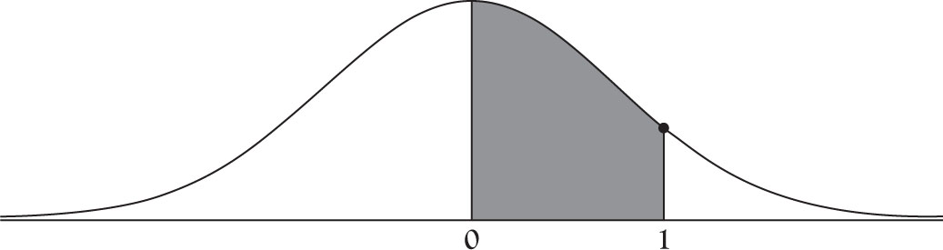
Figure 4.2. The area under the normal distribution between 0 and 1.
Area Under a Normal Distribution with Mean Zero and Variance One
To calculate area under a normal distribution, we can use Table A1 from the Appendix. This table is similar to most other normal tables except it is more accurate because it graduates at half of the customary steps of most normal tables. To read the value of 1.0, go to the left margin of the table and identify the row marked 1.0. Then identify the column marked 0. The value at their intersection is 0.3413, which is the probability corresponding to the shaded area between 0, the mean, and point 1, which is one standard deviation away from the mean to the right.
In the above section we stated that about 68%, or a little more than 2/3 of all observations, are within one standard deviation of the center. Since the points on each side of the center are the mirror images of each other, the probability of being one standard deviation below the mean is the same as the probability of being one standard deviation above the mean, and hence equal to 0.3413. Therefore, the probability of being within one standard deviation of the mean is double the amount of 0.6826, or about 68%. Computations of other values are similar.
P (0 < Z < 1.49) = 0.4319
P (0 < Z < 2.63) = 0.4957
P (-1.52 < Z < 0) = 0.4357
For other variations, it is best to graph the area and perform simple algebra to obtain the results.
P (-1.52 < Z < 1.49) = P (-1.52 < Z < 0) + P (0 < Z < 1.49)
= 0.4357 + 0.4319 = 0.8676
See Figure 4.3 for clarification.
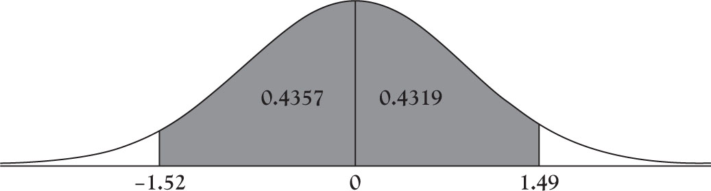
Figure 4.3. Area under normal distribution between -1.52 and 1.49.
P (-1.52 < Z < -1.49) = P (-1.52 < Z < 0) + P (-1.49 < Z < 0)
= 0.4357 - 0.4319 = 0.0038
See Figure 4.4 for finding the shaded area for the last example. Make sure you put the point further away from the center first, because of rules of geometry, and this will guarantee that you would not obtain a negative probability, which does not make any sense.
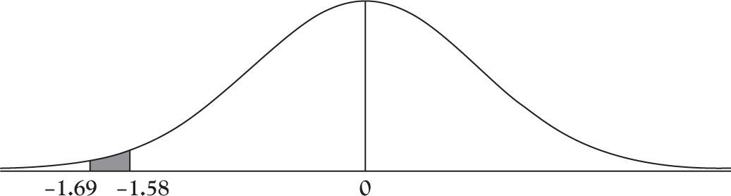
Figure 4.4. Area under normal distribution between -1.69 and -1.58.
Obtaining Probability Values for Normal Distribution with Excel
The above examples can be obtained by using the following command in Excel.
=NORMDIST(1.49,0,1,1) - 0.5 = 0.43188
The formula consists of:
=NORMDIST(X, mean, standard deviation, True)
where “true” represents the “cumulative” value. In this case the entire area under the curve consists of area to the left of the mean, which is equal to half the entire area or 0.5. That is why we are subtracting 0.5 to obtain the area from the mean to point 1.49.
Alternatively, point to the arrow on the side of the “Σ AutoSum” on Excel’s command ribbon and choose “more function.” From the drop-down menu choose “Statistical” in the window labeled “or select a category” and scroll down until you get to NORMDIST command.
Then scroll down until you see NORMDIST. Upon selecting the option, a new window opens up as shown in Figure 4.6.
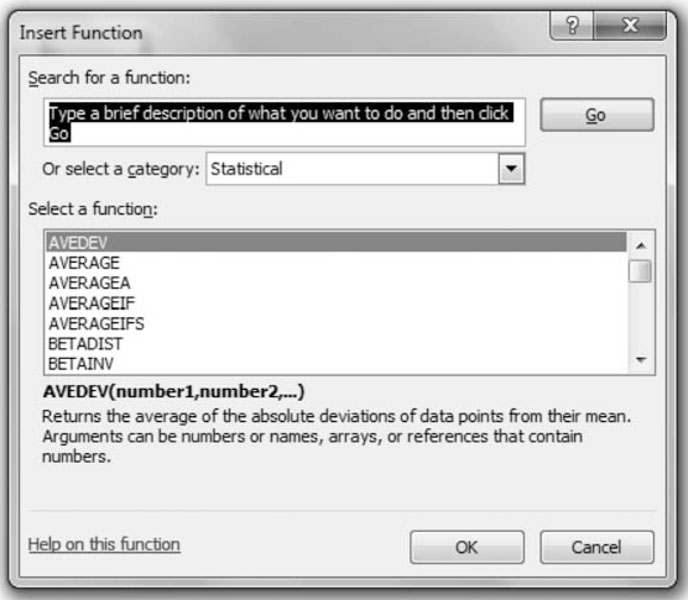
Figure 4.5. Pull-down window for Excel functions.
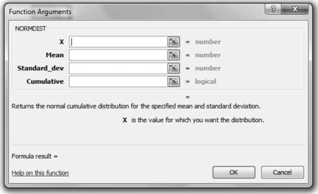
Figure 4.6. Excel window for normal distribution.
Place the appropriate values in the correct boxes and press OK. If you look at the resulting cell, you will see the formula shown previously, except for 0.5, which we added to convert the result to a value between zero and a Z value. When using Excel, write the problem as in the forms shown previously, mark the area under the curve, and then decide if you are subtracting 0.5, adding probabilities, or subtracting them based on the shaded area.
Area Under a Normal Distribution with any Mean and Variance
Convert all normal distributions to the standard normal by standardizing all values.
1.Rewrite the question using probability notations.
2.Convert the values into Z scores. Do not forget the probability.
3.Draw a graph and shade the area under investigation.
4.Look up the probability or use Excel to obtain probability.
When finding the area between two Z values, if Z values are on two sides of zero, that is, one is positive and the other is negative, find the area between 0 and each Z value and add the probabilities. If the Z values are on the same side of 0, that is, either both are negative or both are positive, find the area between 0 and each Z value and subtract the smaller probability from the larger one.
Continuous distribution functions such as normal distribution share two concepts: (1) length and (2) area. The Z score is a measure of length. It shows how far a point is from the center (mean) of standard normal in terms of standard deviations. In other words, Z score indicates the number of units a point deviates from the mean. The probability of a particular Z value from the mean is an area. The area between mean (zero) and a point is the value provided in the standard normal table.
Example 4.1
Assume that the random variable X has a normal distribution with mean 16.9 and standard deviation of 3.01. Find
1.P (X < 22.51)
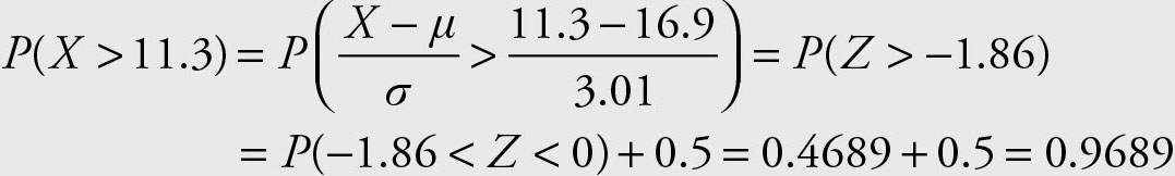
2.P (X > 11.3)
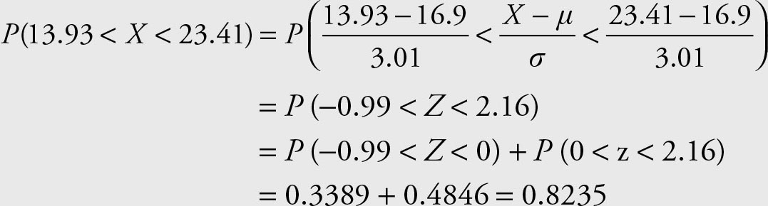
3.P (13.93 < X < 23.41)
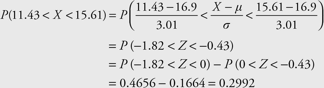
4.P (11.43 < X < 15.61)
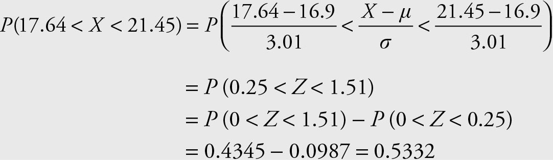
5.P (17.64 < X < 21.45)
Solution
The first step is to standardize the values, both alphabetically and numerically.
1.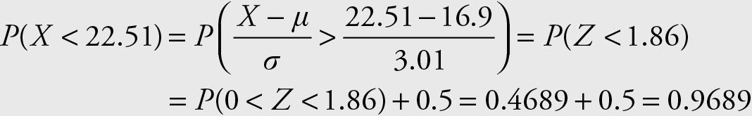
Note that the area of interest is everything to the left of 1.86.
Alternatively, the Excel formula below will give the same answer:
=NORMDIST(22.51, 16.9, 3.01, 1) = 0.9689
2.
Alternatively, the Excel formula below will give the same answer:
=NORMDIST(22.51, 16.9, 3.01, 1) = 0.9689
3.
4.
5.
Example 4.2
Let the random variable X have a normal distribution with mean 15 and standard deviation of 3.
1.What is the cut off value for the top 1% of this population?
2.Find the interquartile range.
Solution
1.In this example, the probability of the outcome is given and the value that determines the desired probability is the objective.
P (Z > z) = 0.01
where the lowercase z represents a specific value. Search for the probability that corresponds to 0.5 - 0.01 = 0.49 in the body of the normal table. The Z score that corresponds to the probability of 0.49 is Z = 2.325.
Next, determine the X value by reversing the computation of the Z score.
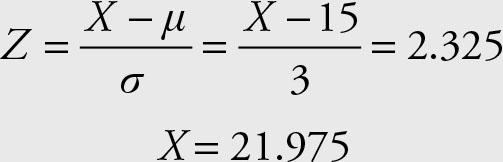
Therefore, 1% of the population has an X value greater than 21.975. Note that 21.975 is the 99th percentile.
2.For the first quartile:
P (Z < - z1) = 0.25
P (-z1 < Z < 0) = 0.5 - 0.25 = 0.25
Search the body of the table for 0.25. The closest number is 0.2502 that corresponds to the Z score of z1 = -0.675. In the Z score formula solve for the value of X.
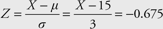
Therefore X = 12.975 is the first quartile.
For the third quartile:
P (Z < z3) = 0.75
P (0 < Z < z3) = 0.75 - 0.5 = 0.25
From the above z3 = +0.675
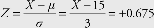
and hence the third quartile is:
X = 17.025
The middle 50% of the population lies between 12.975 and 17.025.
Solution Using Excel
1.Note that in Excel the top 1% is entered as 0.99 for probability.
Point to the arrow on the side of the “Σ AutoSum” on Excel’s ribbon command and choose the “more function.” From the drop-down window choose “Statistical” in the window labeled “or select a category” and scroll down until you get to the NORMINV command (see Figure 4.5).
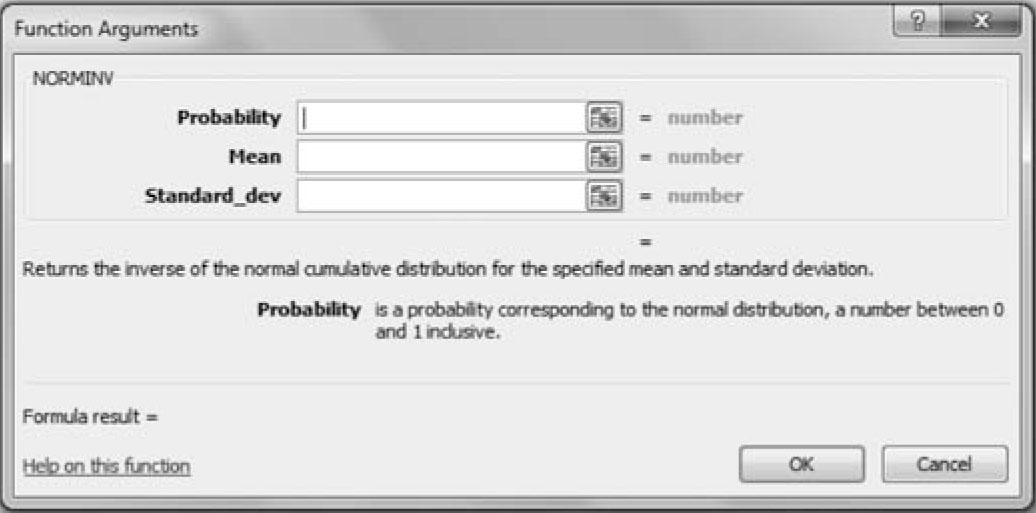
Figure 4.7. Excel window for inverse normal values.
Place the appropriate values in the correct boxes and press OK.
The result 21.97904 is displayed, which is slightly different from the result from the table due to roundoff error. You could have entered the following formula as well.
= NORMINV(0.99,15,3)
2.
= NORMINV(0.25,15,3) = 12.97653
= NORMINV(0.75,15,3) = 17.02347
Again the results are slightly different due to roundoff error. Interestingly, both the above values and the values for the normal distribution table are obtained from Excel.
Nonconformity with Normal Distribution
Normality Versus Skewness
Normal distribution is the cornerstone of statistical analysis. The exact shape of the normal curve depends on the probability density function of the normal distribution. Any deviation from the normal probability density function results in skewness or Kurtosis. It is easy to detect skewness visually because skewed distributions are not symmetric. As a member of continuous symmetric distribution functions, the normal distribution function has the property that its mean, mode, and median coincide. The relationships between these three measures were provided in Chapter 3 for positively and negatively skewed distributions. In the subsequent graph, the positive and negatively skewed functions are superimposed on the normal distribution for comparison.
Normality Versus Kurtosis
Kurtosis measures the degree of flatness or pointedness of a symmetric curve as compared to a normal distribution. There is a formal measure of Kurtosis but involves the concept of the moment of a function which is beyond the scope of this text. However, it is beneficial to depict the graph of a flatter curve, called Platykurtic, which corresponds to a Kurtosis measure with negative value. A more peaked curve, called Leptokurtic corresponds to a Kurtosis measure with a positive value. Figures 4.10 and 4.11 represent comparisons to the normal curve.
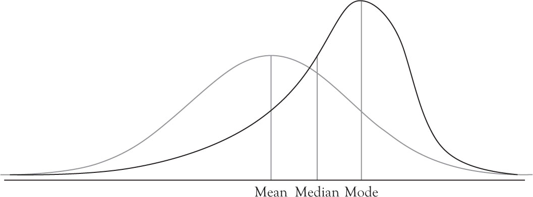
Figure 4.8. Comparison of negative skewness with normal distribution.
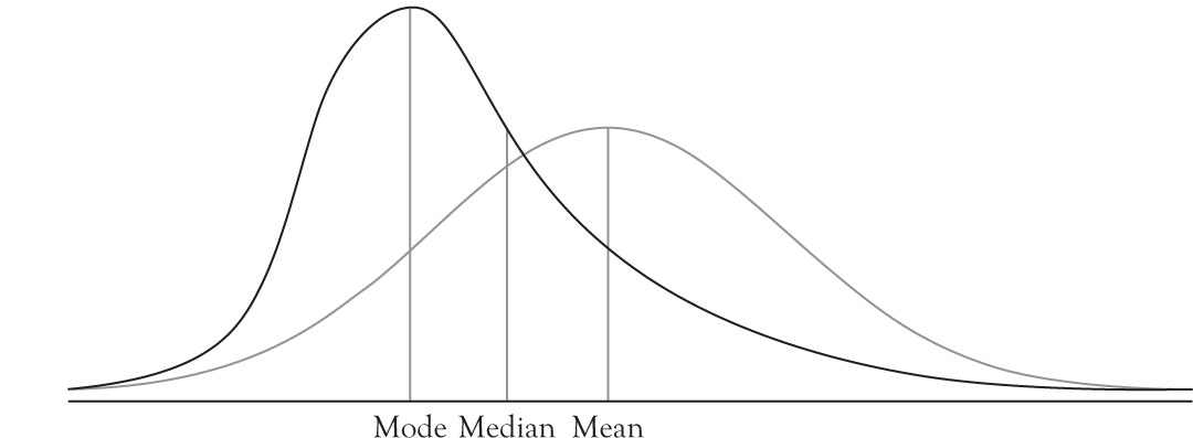
Figure 4.9. Comparison of positive skewness with normal distribution.
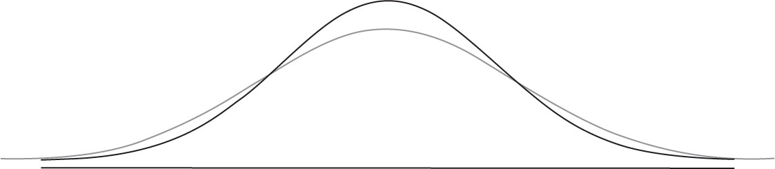
Figure 4.10. Comparison of negative Kurtosis (Platykurtic or flatter) with normal.
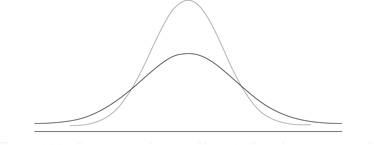
Figure 4.11. Comparison of positive Kurtosis (Leptokurtic or pointed) with normal.
Chi-Squared Distribution Function
Theorem 4.1
Let the random variable X have a normal distribution with mean and positive variance:
X ∼ N (μ, σ2)
Then, the random variable
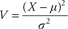
will have a chi-squared (χ2) distribution with one (1) degree of freedom.
V ∼ χ2 (1)
Note that Z = X — μ/σ hence Z2 is a χ2 (1). Therefore, the normal values can be squared to obtain probabilities for the chi-square distribution with 1 degree of freedom.
P (|Z| < 1.96) = 0.956
P (Z 2 < (1.96)2) = P (Z 2 = 3.842) = 0.95
This is identical to the chi-square value with one degree of freedom. Therefore, in confidence intervals and tests of hypotheses one can use either normal distribution or a chi-square distribution. Each one, however, would be beneficial in different settings.
Theorem 4.2
Let X1, X2, . . ., Xn be a random sample of size n from a distribution N (μ, σ2). Recall
Therefore
i. 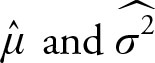 are independent.
ii. 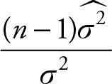 is distributed as a chi-squared with (n - 1) degrees of
freedom.
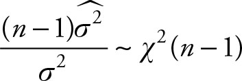
The chi-square distribution is a special case of a gamma distribution. In a gamma distribution with parameters a and θ, let α = r/2 and θ = 2 where r is a positive integer. The resulting distribution function will be a chi-square distribution with r degrees of freedom. The mean will be r and the variance will be 2r.
t Distribution Function
Theorem 4.3
Let X be a random variable that is N (0, 1), and let U be a random variable that is χ2(r). Assume Z and U are independent. Then
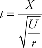 (4.1)
(4.1)
has a t distribution with r degrees of freedom.
Theorem 4.4
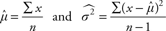
Let X be a random variable that is N (μ, σ2). Use the customary hat-notation to represent sample mean and sample variance. Then the following relationship has a t distribution with (n - 1) degrees of freedom.
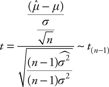 (4.2)
(4.2)
When population variance is not known, using normal distribution for inference is misleading. The problem is more acute when the sample size is small.
F Distribution Function
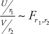
Theorem 4.5
Let U and V be independent chi-square variables with r1 and r2 degrees of freedom, respectively. Then
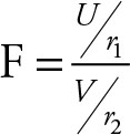 (4.3)
(4.3)
has an F distribution with r1, r2 degrees of freedom.
The relation between F and Z is that
F = e2Z(4.4)
The F Statistics consists of the ratio of two variables, each with a chi-squared, χ2, distribution divided by their corresponding degrees of freedom.