Estimation Versus Inference
There are two distinct ways of using statistics: Descriptive statistics and inferential statistics. Descriptive statistics provide summary statistics in the forms of tables, graphs, or computed values. We can use descriptive statistics to describe population data or sample data. Inferential statistics is used to draw conclusions about population parameters using sample statistics. Obtaining sample statistics for inferential statistics is the same as obtaining them for descriptive statistics. The use of the sample statistics determines whether it is descriptive or inferential. The statistics obtained from a sample for the purpose of inference is called estimation, to emphasize the fact that they are estimates for their respective parameters. In the previous chapters, the portions of descriptive statistics that dealt with samples are actually estimations. When we obtain sample mean, proportion, or variance we are calculating estimates of the corresponding population parameters. As we have demonstrated earlier, estimation is important. When sample estimates are used to test population parameters and to indicate how far the estimates are from parameters, then we are in the domain of inferential statistics. Some statisticians believe that the primary objective of statistics is to make inferences about population parameters using sample statistics. Using sample statistics to make deductions about population parameters is called statistical inference. Statistical inference can be based on point estimation or confidence interval, both of which will be covered shortly. They are closely related, and in some cases, they are interchangeable.
Point Estimation
A point estimate is the statistic obtained from a sample. The reason for the name is because the estimate consists of a single value. Examples of point estimates include sample mean ![]() , sample proportion
, sample proportion ![]() , sample variance
, sample variance  and sample median. These statistics are used to estimate the population mean (μ), population proportion (π), and population variance (σ2), respectively. Sample median can be used to estimate, both, population median and population mean. In fact, any single-valued estimate obtained from a sample is a point estimate. Good estimates are close to the corresponding population parameter. Proper sampling provides accurate estimates of the unknown population parameter. Descriptive statistics addresses the procedure to obtain and calculate point estimates from the sample. It also explains their properties and uses. As discussed in Chapter 3, a suitable estimate is unbiased, consistent, and efficient.
Although point estimates are useful in providing descriptive information about a population, their usefulness is limited because we cannot determine how far they are from the targeted parameter. In order to provide levels of confidence and a probability for margin of error one needs to know the distribution function of sample statistics. Once a sampling distribution of the sample statistic is known, the probability of observing a certain sample statistic can be calculated with the aid of the corresponding table.
Example 6.1
Calculate point estimates of mean, median, variance, standard deviation, and coefficient of variation for the stock prices of Wal-Mart and Microsoft from March 12 to March 30, 2012.
Solution
The solutions are found by using Microsoft Excel. Refer to the Appendix on Excel.
|
Date |
WMT |
MSFT |
|
12 Mar. |
$60.68 |
$32.04 |
|
13 Mar. |
$61.00 |
$32.67 |
|
14 Mar. |
$61.08 |
$32.77 |
|
15 Mar. |
$61.23 |
$32.85 |
|
16 Mar. |
$60.84 |
$32.60 |
|
19 Mar. |
$60.74 |
$32.20 |
|
20 Mar. |
$60.60 |
$31.99 |
|
21 Mar. |
$60.56 |
$31.91 |
|
22 Mar. |
$60.65 |
$32.00 |
|
23 Mar. |
$60.75 |
$32.01 |
|
26 Mar. |
$61.20 |
$32.59 |
|
27 Mar. |
$61.09 |
$32.52 |
|
28 Mar. |
$61.19 |
$32.19 |
|
29 Mar. |
$60.82 |
$32.12 |
|
30 Mar. |
$61.20 |
$32.26 |
|
Mean |
$60.89 |
$32.32 |
|
Variance |
0.056464 |
0.10941 |
|
Median |
$60.83 |
$32.20 |
|
St. Dev |
0.237622 |
0.33078 |
|
CV |
$0.0039 |
$0.0102 |
Interval Estimation
Statistics deals with random phenomena. Nothing remains constant in life. Methods of production change. Processes are modified. Machines get out of calibration. New techniques are applied. In all these cases, statistics is used to determine what remains constant and what changes. In estimation theory, sample statistics is used to estimate the population parameter. However, when one uses point estimation, it is not clear how close the estimate is to the parameter and there is no measure of confidence. This does not mean that point estimates are useless or unreliable. With proper sampling the point estimates will be unbiased, consistent, and efficient.
Interval estimation augments point estimates by providing a margin of error for the point estimate. The margin of error is a range, based on the degree of certainty, for the estimate of the population parameter, which is added and subtracted from a point estimate. Confidence intervals are based on the point estimate of the parameter and the distribution function of the point estimate. It is affected by the level of certainty, the variance of data, and the sample size.
Calculating Confidence Intervals
Interval estimation is a simple notion and is defined as:
Point estimate ± Margin of error(6.1)
In order to explain this concept we need to recall things from Chapters 2, 3, and 4. We covered point estimates in Chapter 2, although we did not use the same terminology. Point estimates are sample statistics and are used to estimate the corresponding population parameters. Mean, median, variance, and proportion are some common examples of point estimates.
The margin of error is not totally new either. It is based on the use of Z score, which we covered in Chapter 3. In Chapter 4 we introduced the normal distribution function and demonstrated the use of Z score and standardization in obtaining probabilities of random variables from normal distribution. Also in Chapter 4, we used a Z score to obtain the probability under normal distribution between two points. Previously we pointed out that due to symmetry of the standardized normal distribution, the probability of the area from zero, that is, the center, to a point on the right is equal to the probability of the area from zero to the negative value of that number (see Figure 6.1).
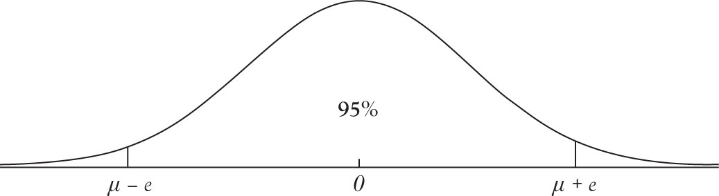
Figure 6.1. Margin of error on normal distribution.
Note that in Figure 6.1, the mean is 0 and the standard deviation is 1. Also recall that the unit of measurement of the Z score is the standard deviation. Conventionally, we do not write 1 but if the standard deviation was different from 1, we must include that in the measure, as in Figure 6.1. Therefore, a point on the normal distribution curve is ZΣ away from the mean.
When dealing with sample statistics, the properties of sampling distribution apply. Therefore, in the case of statistics, that is, estimates obtained from the sample, the Central Limit Theorem states that the standard deviation is given by 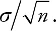 Replacing σ with the this formula provides
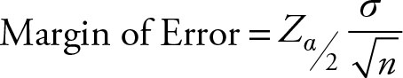 (6.2)
(6.2)
It is very important to realize that the margin of error formula in Equation 6.2 depends on the knowledge of population variance. When the population variance is unknown and the sample variance has to be used, then the formula must be adjusted by replacing the population standard deviation with the sample standard deviation and the Z value must be replaced by the t value as in Equation 6.3:
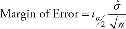 (6.3)
(6.3)
Example 6.2
Calculate the margin of error for Microsoft stock price for the period March 12–March 30, 2012, using 83% level of confidence. Assume the real population variance is equal to the sample variance.
Solution
First obtain the Z value that corresponds to half of the 0.83 level of confidence so we can use the normal table provided in the Appendix to this book.

Searching in the body of the normal table, we find the probability 0.415 corresponds roughly to Z = 1.375. Note that we are using the sample variance as if it was the actual population variance.
According to Example 2.16 the variance of the data is 0.102.
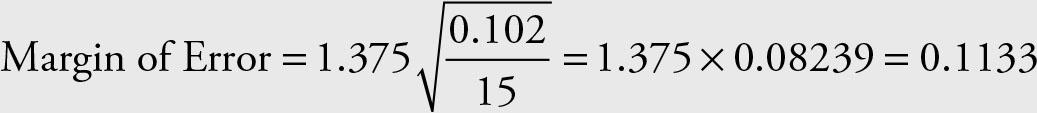
However, since the population variance is unknown we must use the t value instead of Z value. Unfortunately, t values for alpha of (1 – 0.83)/2 = 0.085 are not readily available. However, Microsoft Excel provides the necessary number by using the following command:
= t.inv(0.085, 14) = 1.44669
Note that Excel will provide a negative sign in front of the t value because it refers to the left hand tail. But we do not need to worry, since the distribution is symmetric.
Therefore, Margin of Error = 1.44669 × 0.2316 = 0.33505
This is the correct value of margin of error because it is using the t value, as required when population variance is unknown.
The concept of margin of error applies to sample statistics but not to the population parameters. Population parameters are constant values and do not have margin of error. However, sample statistics, which are random variables and are estimating their respective population parameters, have a margin of error. As seen in Equation 6.2, margin of error is directly related to variance of the population and the level of confidence, as indicated by the Z score, and inversely related to the square root of the sample mean.
Recall from Chapter 5 that the sampling distribution of sample mean is affected by the knowledge of the population variance. If the population variance is known, the distribution function of the sample mean is a normal distribution. However, if the population variance is not known the distribution function of the sample mean is a t distribution. Therefore, when calculating the margin of error we must use either the normal table or the t table, depending on whether the population variance is known or unknown, respectively.
In Chapter 5, we learned the sampling distribution function of one sample statistics such as mean, proportion, and variance. When calculating margin of error for these statistics we need to use the appropriate distribution function. We learned the sampling distribution of the differences of two sample means and two sample proportions, both of which are a normal distribution. We also learned the sampling distribution of two variances, which is an F distribution. Once the margin of error is calculated, obtaining confidence interval is simple by using Equation 6.1.
Terminology
The probability between –Z and +Z from a standard normal, that is, a normal distribution with mean zero 0 and variance 1, is shown by (1 – a)%. This is because the area outside of the above range is equal to a. In Chapter 7, we will provide more explanation for the naming of these areas and go into more detail on the meaning of the term a.
Customarily, normal distribution tables are calculated for half of the area, because of symmetry. Thus, the Z value, which corresponds to one half of a is shown as 
Interval Estimation for One Population Mean
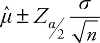
The correct way of writing interval estimation of Equation 6.1 when estimating the population mean is
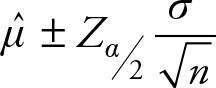 (6.4)
(6.4)
Definition 6.1
Based on Chapter 5, the (1 – a)% confidence interval for the mean of one population (m) when the population variance is known is given by Equation (6.4).
Note that we need to calculate the following two values to obtain a confidence interval.
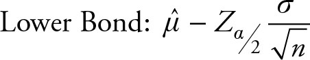 (6.5)
(6.5)
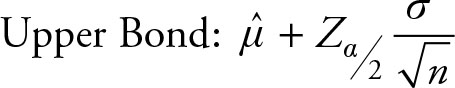 (6.6)
(6.6)
Sometimes we refer to the lower bond and upper bond as LB and UB, respectively.
Rule 6.1 Inference with Confidence Interval
The confidence interval covers the true population parameter with (1– a)% confidence.
Example 6.3
Provide an 83% confidence interval for Microsoft stock price for the period of March 12 to March 30, 2012. Assume the real population variance is equal to the sample variance.
Solution
From Examples 6.1 and 6.2 we have the necessary numbers.
LB = 32.32 − 0.1133 = 31.21
UB = 32.32 + 0.1133 = 32.43
An 83% confidence interval for the mean of Microsoft stock price between March 12 to March 30, 2012, is given by the range $31.21 to $32.43.
Note that we assumed the sample variance is equal to the population variance in order to apply the example to this case. If the variance is unknown, which is true more often than it is not, we have to use Equation 6.7. Furthermore, when the value of population variance is not known, we must use a t distribution value rather than a Z distribution value.
Definition 6.2
Based on Chapter 5, the (1 – a)% confidence interval for the mean of one population (m) when the population variance is unknown, is given by the following equation:
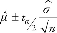 (6.7)
(6.7)
In earlier days when t tables were only available for 1%, 5%, and 10% levels of significance, most researchers would use a normal table instead of the t table when sample size was greater than 30. With wide availability of t values for any level of significance, this practice is no longer necessary.
Example 6.4
Provide a 95% confidence interval for Microsoft stock price for the period of March 12 to March 30, 2012.
Solution
Since the population variance is unknown and the sample size is less than 30, we need to use the t distribution. The t value for 95% confidence interval is ±2.14479. To obtain this value look under 2.5% probability of type I error with 14 degrees of freedom in the t table or use the following Excel command.
= t.inv(.025,14) = −2.14479
The value reported by Excel is negative because it is designed to report the lower-end critical value.
Example 6.2 reported the appropriate standard deviation based on the variance calculated in Example 1.16.
LB = 32.32 – 2.14479 (0.8239) = 30.55291
UB = 32.32 + 2.14479 (0.8239) = 34.08709
A 95% confidence interval for the mean of Microsoft stock price is given by the range $30.55 to $34.09. This is the correct confidence interval because it uses the t value since the population variance is unknown.
Since t values are somewhat larger, to account for the fact that the population variance is unknown and must be estimated, the corresponding confidence interval is wider than the one calculated using a Z table when we assume to know the population variance.
Definition 6.3
Based on Chapter 5, the (1 – a)% confidence interval for the proportion of one population (π) is given by the following equation:
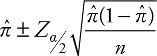 (6.8)
(6.8)
Example 6.5
Calculate a 95% confidence interval for the proportion of stock prices of Microsoft that are higher than $32.5. Use the sample data from April 2 to April 21, 2012, provided in Example 3.2.
Solution
The sample proportion of stocks over $32.5 is
The Z value corresponding to 95% confidence is 1.96.
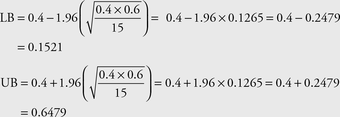
The range 0.1521 to 0.6479 covers the true population proportion of Microsoft stock prices that are $32.5 or higher.
Since the population variance is not known and the sample size is smaller than 30, we should have used the t distribution instead of normal distribution. In practice, the sample size is much larger when proportions are used. The results using the t values are given by:
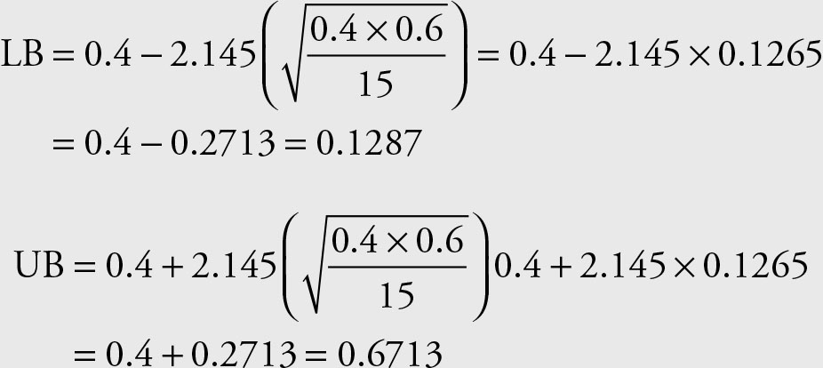
The range 0.1287 to 0.6713 covers the true population proportion of Microsoft stock prices that are $32.5 or higher. Note that the range became wider when we used the t distribution value. This is the consequence of not knowing the population variance.
Definition 6.4
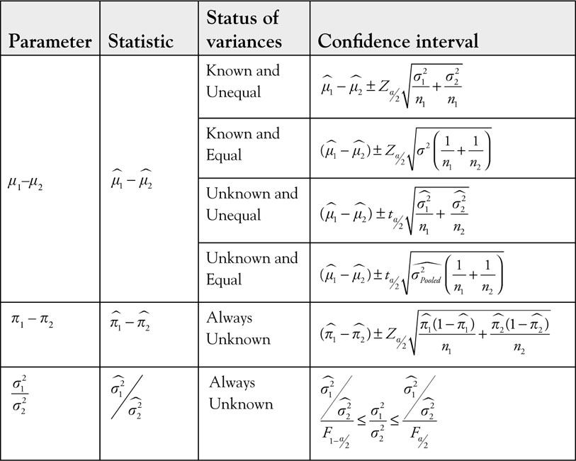
Based on Chapter 5, the (1 – a)% confidence interval for the difference of means of two populations (μ1 – μ2) when the population variances are known and unequal is given by the following equation:
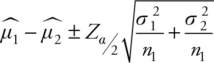 (6.9)
(6.9)
Definition 6.5
Based on Chapter 5, the (1 – a)% confidence interval for the difference of means of two populations (μ1–μ2) when the population variances are known and equal is given by the following equation:
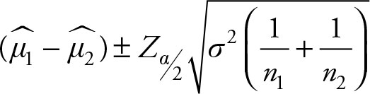 (6.10)
Definition 6.6
Based on Chapter 5, the (1– a)% confidence interval for the difference of means of two populations (μ1–μ2) when the population variances are unknown and unequal is given by the following equation:
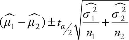 (6.11)
Example 6.6
Obtain a 95% confidence interval for the difference in Microsoft stock prices between March 12 and March 30, 2012, and April 2 and April 21, 2012. The data is provided in Example 3.2.
Solution
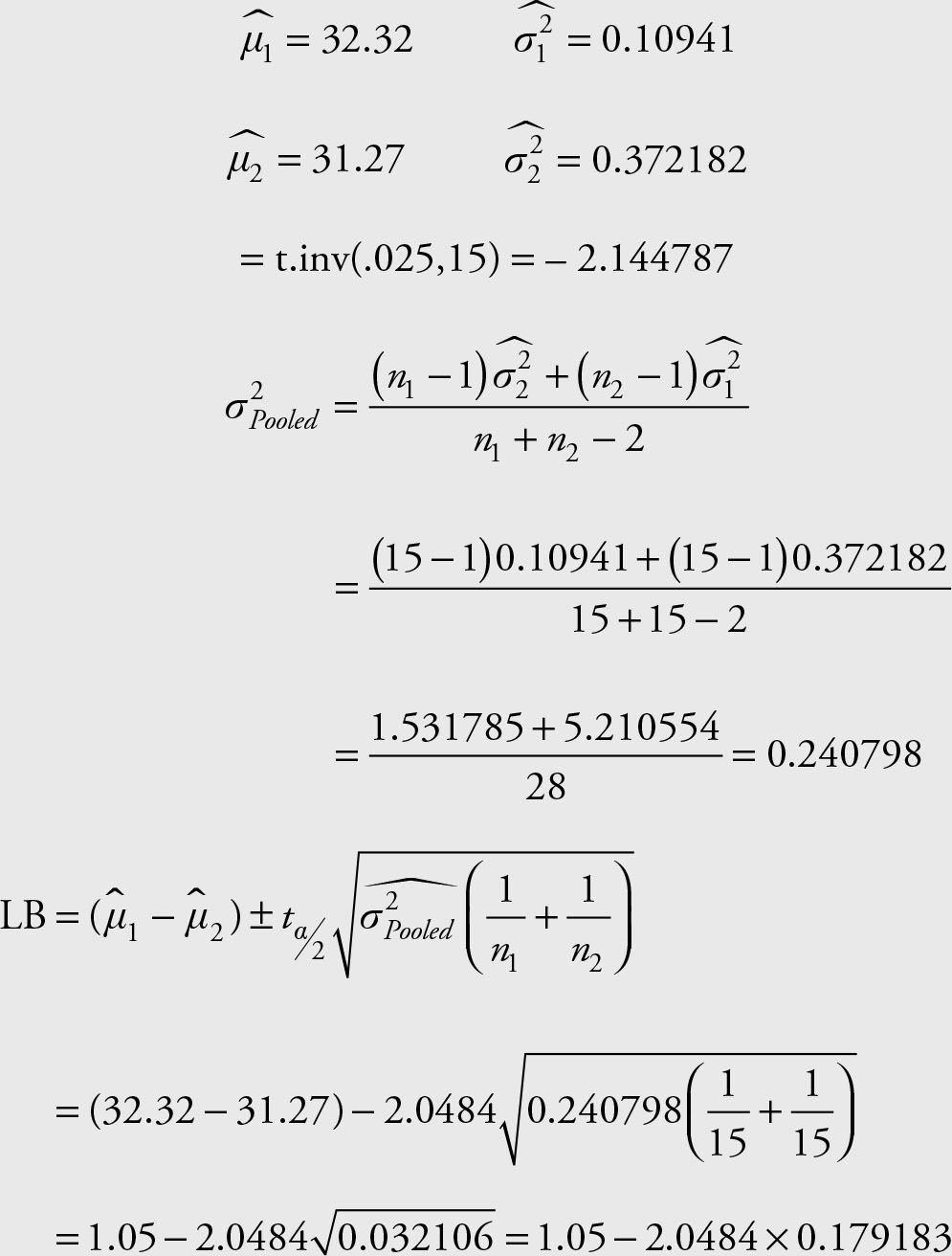
Let’s mark the data in March with the subscript “1” and those for April with subscript “2.” The required formula is given in Equation 6.11. According to the formula we need the means and variances from both periods as well as the t value corresponding to 95% confidence.
We have the following results from previous examples. Make sure to verify the accuracy of the output. Remember that rounding off the numbers in early stages of calculation may produce discrepancies in final results. Here, we are using the output from Excel, which is somewhat larger than the values obtained using the computational method of Equation 2.35. The short-cut Equation 2.35 produces the least amount of rounding off, and thus is more accurate.
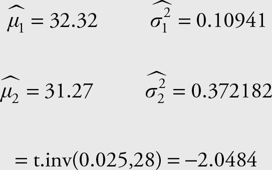
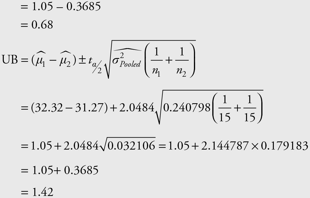
Since we lose two degrees of freedom the correct degrees of freedom for the t distribution is 15 + 15 - 2 = 28. Recall that we need to use both positive and negative t values.
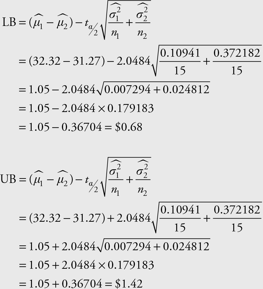
The range $0.68 to $1.42 covers the difference of the means of the two periods of stock prices for Microsoft with 95% probability.
Definition 6.7
Based on Chapter 5, the (1 – a)% confidence interval for the difference of means of two populations (μ1 – μ2) when the population variances are unknown and equal is given by the following equation:
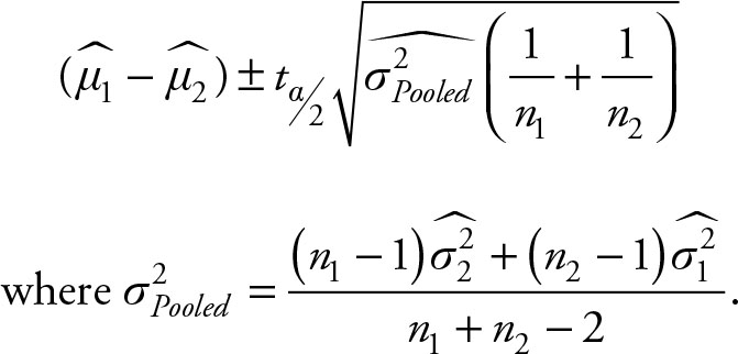 (6.12)
Example 6.7
Obtain a 95% confidence interval for the difference in Microsoft stock prices between March 12 and March 30, 2012, and April 2 and April 21, 2012. The data is provided in Example 3.2.
Solution
Since the data belongs to the same company and are so close in time period, it is reasonable to assume that there is one variance for the company’s stock prices and the two sample statistics are two estimates of the same population variance. Therefore, it is necessary to find their weighted averages and then use Equation 6.12. We already have the following results:
The range $0.68 to $1.42 covers the difference of the means of the two periods of stock prices for Microsoft with 95% probability.
The reason these results are exactly the same as the result for the previous case, where we did not assume the equality of the variances, is that the two sample sizes are equal. When samples have different sizes the results will be different.
Definition 6.8
Based on Chapter 5, the (1 – a)% confidence interval for the difference of two population proportions (π1 – π2) is given by the following equation:
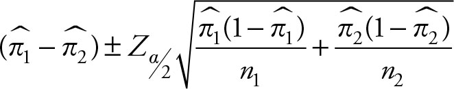 (6.13)
Example 6.8
Calculate a 95% confidence interval for the difference of the proportion of stock prices of Microsoft that are more than or equal to $32.00 for the periods March 12–30, 2012, and April 2–21, 2012; the data is provided in Example 3.2.
Solution
Let’s mark the data in March with the subscript “1” and those for April with subscript “2.” The sample proportion of stocks more than or equal to $32.00 for each period is given by:
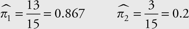
The Z value corresponding to 95% confidence is 1.96. Insert these values in Equation 6.13 to obtain the results.
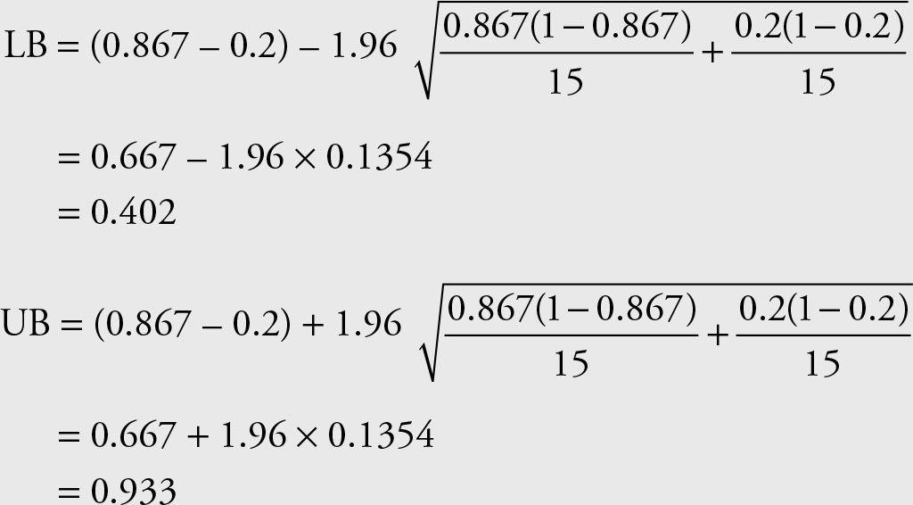
The range from 0.402 to 0.933 covers the difference of the ratios of stock prices for Microsoft that is greater than or equal to $32.00 in the two periods March 12–30 and April 2–21.
Definition 6.9
Based on Chapter 5, the (1– a)% confidence interval for one population variance (σ2) is given by the following equation:
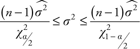 (6.14)
Note that the chi-squared distribution is not symmetric, therefore we cannot use the ± signs to form the confidence interval. Also, it is important to note that the term  refers to the right side of the distribution and, hence, it is larger than
 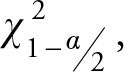 which refers to the left side of the distribution. Dividing the same numerator by a larger number provides a smaller result, hence the lower bond; while dividing the same numerator by a smaller value gives a larger result, hence the upper bond.
Example 6.9
Find the 95% confidence interval for the variance of stock prices for Microsoft. Use the sample data for the period April 2–21, 2012, provided in Example 3.2.
Solution
The sample variance for April 2–21 and the chi-squared values for 0.025 and 0.975 with 14 degrees of freedom are:
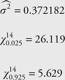
Use Equation 6.14 to build the confidence interval
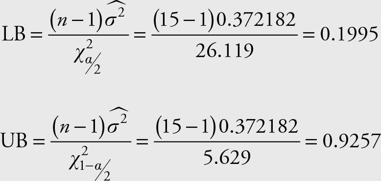
The range 0.1995 to 0.9257 covers the population variance of Microsoft stock prices with 95% confidence.
Definition 6.10
Based on Chapter 5, the (1– a)% confidence interval for the ratio of two population variances 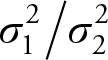 is given by the following equation:
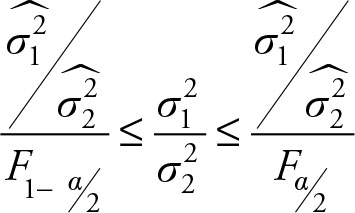 (6.15)
Note that since the F distribution is not symmetric, we cannot use the ± signs to form the confidence interval. Also, it is important to note that term  refers to the right side of the distribution and, hence, it is larger than
  which refers to the left side of the distribution. Dividing the same numerator by a larger number provides a smaller result, hence the lower bond, while dividing the same numerator by a smaller value gives a larger result, hence the upper bond.
Example 6.10
Find the confidence interval for the ratio of the variances for the two periods March 12–30, 2012, and April 2–21, 2012, for Microsoft stock prices.
Solution
Let’s mark the data for March with the subscript “1” and those for April with subscript “2.” The variances and the F values for 0.025 and 0.975 with 14 degrees of freedom are:
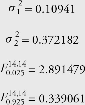
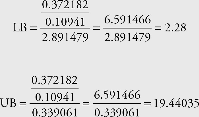
The range 2.28 to 19.44035 covers the ratio of variances for the two periods for Microsoft stock prices with 95% confidence.
Since the confidence interval does not cover the value “1,” it is unreasonable to believe that the variances of the two periods are the same. We will address this in more detail in Chapter 7, when we discuss the test of hypothesis. In light of this finding, we should use Equation 6.9 when testing equality of the means for the two periods, as in Example 6.6.
Determining the Sample Size
In Chapter 4 we showed the necessary sample size for estimating the single mean of a population. The sample size in that case was obtained by algebraic manipulation of the margin of error in Equation 6.4, which is repeated below for your reference.
 (6.4)
(6.4)
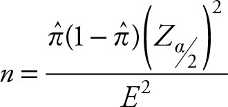
Setting the margin of error equal to a desired margin of error, E, and solving for n results in the following formula:
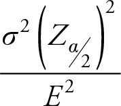 (6.16)
Example 6.11
What size sample is needed to be within $0.10 of the actual price if the variance is 0.372182 with 95% confidence?
Solution
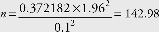
Therefore, the necessary sample size is 143. Note that the variance in this formula is the population variance. When the population variance is unknown, use the sample variance instead, but remember to use the t value instead of the Z value.
Similar algebraic manipulations are applied to obtain sample sizes for cases with unknown variances, involving, both, the one or two population means, proportions, and variances. We will only show the results for one population proportions for reference.
 (6.17)
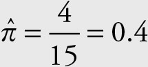
Example 6.11
What size sample is needed to be within 5% of the population proportion with 95% confidence when the sample proportion is 0.4?
Solution
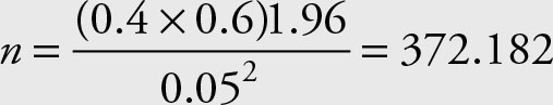
Therefore, the necessary sample size is n = 369.
Inference with Confidence Intervals
The primary objective of statistics is to make inferences about population parameters using sample statistics. Using sample statistics to make deductions about population parameters is called statistical inference. Statistical inference can be based on point estimation, confidence interval, or test of hypothesis. These are closely related and in some aspects they are interchangeable. The inference can be based on the estimation theory or decision theory. Test of hypothesis is a tool for decision theory. The estimation theory consists of point estimation and interval estimation. This section will deal with the confidence interval.
Population parameters are unknown and constants. Sample statistics, which are random by nature, are used to provide estimates of population parameters. If sampling is random, then the sample statistics is a good estimate of the corresponding population parameter. A good sample statistics has desirable properties, as discussed in Chapter 3. These statistics are called point estimates because they provide a single value as the estimate of the population parameter. If the estimator is “good” then it should be close to the unknown true value of the population parameter. The single estimate does not indicate proximity to the true parameter or probability of being close to the true parameter. Confidence intervals give, both, an idea of actual value of population parameter and also a probability, or a level of confidence, that the interval includes the population parameter.
Table 6.1. Summary of Confidence Interval for One Population
Parameter

Table 6.2. Confidence Interval for Two Samples