
Statistical Inference with Test of Hypothesis
Choose Evidence with High Probability
One of the methods of drawing inference about population parameters using sample statistics is by testing the hypothesis about the parameters. With proper sampling techniques, a point estimate provides the best estimate of the population parameter. Interval estimation provides a desired level of probability of level of confidence in the estimate. Test of hypothesis is used to make assertions on whether a hypothesized parameter can be refuted based on evidence from a sample.
Using sample statistics to make deductions about population parameters is called statistical inference. Statistical inference can be based on point estimation, confidence interval, or test of hypothesis. They are closely related and in some aspects they are interchangeable. This section will deal with test of hypothesis. The technical definition of a hypothesis is based on the distributional properties of random variables.
The purpose of test of hypothesis is to make a decision on the validity of the value of a parameter stated in the null hypothesis based on the observed sample statistics. Recall that parameters are constant and unknown while statistics are variable and known. You calculate and observe the statistics. If the observed statistics is reasonably close to the hypothesized value, then nothing unexpected has happened and the (minor) difference can be attributed to random error. If the observed statistics is too far away from the hypothesized value, then either the null hypothesis is true and something unusual with very low probability happened, or the null hypothesis is false and the sample consists of unusual observations. Following sampling procedures and obtaining a random sample reduces the chance of an unusual sample, which may still occur in rare occasions. Therefore, proper sampling assures that unusual sample statistics have low probabilities. On the other hand, sample statistics representing the more common possibilities would have a high probability of being selected.
Statistical inference consists of accepting outcomes with high probability and rejecting outcomes with low probability. If the
sample statistics does not contradict the hypothesized parameter, then the hypothesized parameter should not be rejected. If the probability of observed statistics is low we reject the null hypothesis; otherwise we fail to reject the null hypothesis. In order to find the probability of an occurrence for sample statistics we need to know its sampling distribution.
Hypothesis
A hypothesis is formed to make a statement about a parameter. Although in English language terms such as “statement” and “claim” may be used interchangeably, in statistics, as will be explained shortly, we use the word “claim” only about the alternative hypothesis.
Definition 7.1
A statistical hypothesis is an assertion about the distribution of one or more random variables. When a hypothesis completely specifies the distribution, it is called a simple statistical hypothesis; otherwise, it is called a composite statistical hypothesis.
Hypotheses are customarily expressed in terms of parameters of the corresponding distribution function. If the parameter is set equal to a specific value it is a simple hypothesis; otherwise it is a composite hypothesis. For example, the hypothesis that the average price of a particular stock is $33.69 is written as μ = 33.69. This is a simple hypothesis. However, the hypothesis that the average price of a particular stock is less than $33.69 is written as μ < 33.69. This is a composite hypothesis because it does not completely specify the distribution.
Definition 7.2
When the hypothesis gives an exact value for all unknown parameters of the assumed distribution function, it is called a simple hypothesis; otherwise the hypothesis is composite.
In this text we deal with the simple hypothesis exclusively.
Null Hypothesis
The null hypothesis reflects the status quo. It is about how things have been or are currently. For example, the average life of a car is 7 years. The null hypothesis can be a statement about the nature of something, such as, “an average man is 5'10" tall.” The null hypothesis might be the deliberate setting of equipment, such as, “a soda-dispensing machine puts 12 ounces of liquid in a can.” A statistical hypothesis is not limited to the average only. We can have a hypothesis about any parameter of a distribution function, such as, 54% of adults are Democrats; the variance for weekly sales is 50. The symbol for a null hypothesis is H0, pronounced h-sub-zero. The following represent the previous examples in the customary notation of the hypothesis. Note that the stated null hypotheses are simple hypotheses as we will only address tests of simple hypotheses.
Single Mean
H0: μ = 7
H0: μ = 5'10"
H0: μ = 12
Single Proportion
H0: π = 0.54
Single Variance
H0: σ2 = 50
In summary, the null hypothesis is a fact of life, the way things have been, or a state of nature. This includes the setting of machinery, or deliberate calibration of equipment. If the fact of life, the state of nature, the setting of machinery, the calibration of equipment has not changed, or there is no doubt about them, then the null hypothesis is not tested. When you purchase a can of soda that states it contains 12 ounces of drink you do not check to see if it does actually contain 12 ounces; you have no doubt about it, so you do not test it. Many such “null hypotheses” are believed to be true and, hence, not tested. It is tempting to state that the manufacturer is making the “claim” that the can contains 12 ounces; however, their statement is more of an assertion or a promise and not a claim. As we will see shortly, the alternative hypothesis is the claim of the researcher, which is also known as the research question. The null hypothesis for a simple hypothesis is always equal to a constant. The format is:
H0: A parameter = A constant(7.1)
In order to test a hypothesis, we either have to know the distribution function or the random variables. If the distribution function has more than one parameter, we need to know the other parameter(s); otherwise we will be dealing with a composite hypothesis.
In a hypothesis, testing the expected value of the outcome of an experiment is the hypothesized value. The hypothesized value reflects the status quo and will prevail until rejected. In practice, the observed value is indeed a statistics obtained from a sample of reasonable size. Care must be taken.
When testing a hypothesis about variance, note that the constant  should be a non-negative number. In practice, zero variance is not a reasonable choice and the value is usually positive. This parameter is different than the mean or proportion, and it has a chi-squared distribution. Therefore, its test statistics will be very different from the others.
Null Hypothesis for Equality of Two Parameters
The test of hypothesis can be used to test the equality of parameters from two populations. Let θ1 and θ2 be two parameters from two populations. With no prior information the two parameters would be assumed to be the same until proven otherwise. For example, the average productivity of a man and a woman would be the same until proven otherwise. The null hypothesis should not be written as:
H0: θ1 = θ2(7.2)
This hypothesis is setting one parameter equal to the other, which makes it a composite hypothesis. Using algebra the hypothesis can be modified to convert it to a simple hypothesis. There are two possible modifications. Equation (7.2) can be written in the following two forms.
H0: θ1 − θ2 = 0, or(7.3)
 (7.4)
(7.4)
The only thing that remains to be established is that the difference of two parameters or the ratio of two parameters is also a parameter, and that we have an appropriate distribution function to use as test statistics. We have accomplished these in Chapter 5, but will reinforce them in this chapter as well.
Null Hypothesis of Two Means
The representations in Equations 7.3 and 7.4 are to test the equality of two parameters. Depending on the parameters, we may use one or the other representation based on availability of a distribution function. In Chapter 5, we showed appropriate distribution functions for the difference of two means of random variables, each with a normal distribution. The difference of two means from a normally distributed function is a parameter, and if the two are equal, their difference will be zero. This will allow the use of normal distribution for testing the following hypothesis, which is identical to H0: μ1 = μ2.
H0: μ1 − μ2 = 0(7.5)
Null Hypothesis of Two Proportions
In Chapter 5, we showed that if a population has a normal distribution with proportion π1 and another population has a normal distribution with proportion π2, the difference of the two parameters will also have a normal distribution with the proportion π1 − π2. The difference of the two proportions of two normal populations is a parameter, and if the two are equal, their difference will be zero. This will allow the use of normal distribution for testing the following hypothesis, which is identical to H0: π1 = π2.
H0: π1 − π2 = 0(7.6)
Null Hypothesis of Two Variances ![]()
In Chapter 5, we showed that σ2 has a chi-squared distribution. The ratio of ![]() to
to ![]() , after each is divided by its degrees of freedom, has an F distribution (see Chapter 5). The F distribution will have degrees of freedom associated with the corresponding numerator and denominator chi-squared distributions. The ratio of two variances is a parameter with F distribution, and if they are equal then their ratio will be equal to 1. This will allow the use of F distribution for testing the following hypothesis, which is identical to
, after each is divided by its degrees of freedom, has an F distribution (see Chapter 5). The F distribution will have degrees of freedom associated with the corresponding numerator and denominator chi-squared distributions. The ratio of two variances is a parameter with F distribution, and if they are equal then their ratio will be equal to 1. This will allow the use of F distribution for testing the following hypothesis, which is identical to ![]()
 (7.7)
(7.7)
Alternative Hypothesis
The alternative hypothesis is the claim a researcher has against the null hypothesis. It is the research question or the main purpose of the research. The formation of the null and the alternative hypotheses are the main problem of the novice. Remember the following:
• The null hypothesis is always of this form:
A parameter = A constant when we deal with simple hypothesis.
All of the previous null hypotheses are simple hypothesis.
•The claim might be that the parameter is greater than (>), less than (<), or not equal to (≠) a constant, which reflects the claim that the parameter has increased (>), decreased (<), or it simply has changed (≠).
•Null means something that nullifies something else. Therefore, the null hypothesis is the value that nullifies the alternative hypothesis. In all three cases the relationship that nullifies the (>), (<), and (≠) is the (=) sign.
The alternative hypothesis is designated by H1 and is pronounced h-sub-one or alternative hypothesis. The only time a hypothesis is formed and consequently tested is when there is a doubt about null hypothesis.
How to Determine the Alternative Hypothesis
The claim of the research, that is, the research question, determines the alternative hypothesis. Every alternative hypothesis is a claim that the null hypothesis has changed. When the claim is that the value of parameter in the null hypothesis has declined, then the appropriate sign is the “less than” sign (<). Focus on the meaning and not the wording. When the claim is that the value of the parameter in the null hypothesis has increased, then the appropriate sign is the “greater than” sign (>). These two alternative hypotheses are known as one-tailed hypotheses. When the claim is not specific, or is indeterminate, then the appropriate sign is the “not equal” sign (≠). This is known as a two-tailed hypothesis. None of the three alternative cases include an equal sign (=), because the equal sign nullifies all of the above signs. Furthermore, in order to draw inference at this introductory level, the null hypothesis must be a simple hypothesis, which takes the form H0: A parameter = A constant.
Alternative Hypothesis for a Single Mean
•A consumer advocacy group claims that car manufacturers are cutting corners to maintain profitability and make inferior cars that do not last as long.
H0: μ = 7
H1: μ < 7
•Men are getting taller because of better nutrition and more exercise.
H0: μ = 5'10"
H1: μ > 5'10"
•The quality manager would like to know if the calibration of soda dispensing machine is still correct.
H0: μ = 12
H1: μ ≠ 12
Alternative Hypothesis for a Single Proportion
•A political science researcher believes that due to globalization of the economy and political turmoil around the world, the percentage of Democrats has declined.
H0: π = 0.54
H1: π < 0.54
Alternative Hypothesis for a Single Variance
•Increased promotional advertising has increased the variance of weekly sales.
H0: σ2 = 50
H1: σ2 > 50
The alternative hypothesis is the claim someone has against the status quo. If there is no claim, then there is no alternative hypothesis and, hence, no need for a test. The nature of the claim determines the sign of the alternative. In the alternative hypothesis the parameter under consideration can be less than, greater than, or not equal to the constant stated in the null hypothesis. The sign of the alternative hypothesis depends on the claim and nothing else.
Test Statistics
In Chapter 5 we saw that when statistics is a sample mean ![]() , a sample proportion
, a sample proportion ![]() , two sample means
, two sample means  or two sample proportions
  , the Central Limit Theorem asserts that each of these sample statistics have a normal distribution. Sample variance
  has a chi-squared distribution. The ratio of two sample variances
  has an F distribution. Cases involving two statistics test their equality. The test statistics for single mean (μ), two means (μ1 – μ2), single proportion (π), and two proportions (π1 – π2) is provided by
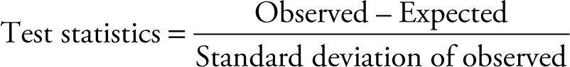 (7.8)
(7.8)
The statistics obtained from the sample provides the observed portion of the formula. The null hypothesis provides the expected value. The other name for standard deviation of the observed value is standard error. The Central Limit Theorem provides the distribution function and the standard error. The sampling distribution of sample statistics covered in Chapter 5 provides a summary of parameters, statistics, and sampling variances of one and two populations. Whether the correct statistics for this hypothesis is Z test or t test depends on whether the population variance is known. Use the Z test when the population variance is known, or when it is unknown and sample size is large. Note that Z statistics can only be used to test hypothesis about one mean, one proportion, two means, or two proportions. In the case of two means or two proportions, the hypotheses must be modified to resemble a simple hypothesis. Use t statistics when the population variance is unknown and sample size is small. Note that t statistics can only be used to test hypotheses about one mean, one proportion, two means, or two proportions.
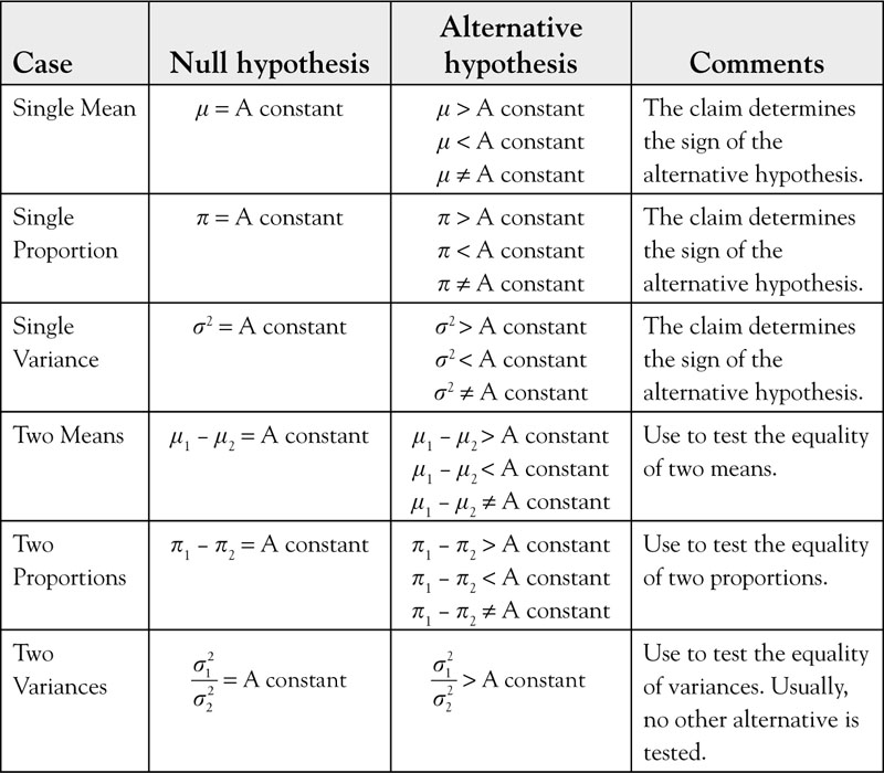
Table 7.1. Summary of Null and Alternative Hypothesis
The test statistics for a single variance (σ2) is given by
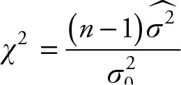 (7.9)
(7.9)
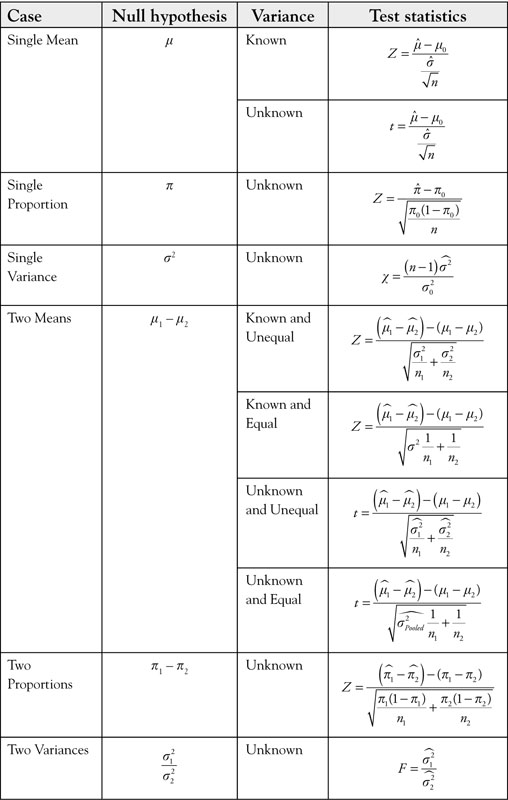
The test statistics for equality of two variances is given by
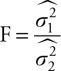 (7.10)
The actual tests are provided in Table 7.2, which is a summary of tools developed in Chapters 5, 6, and 7.
Table 7.2. Test Statistics for Testing Hypotheses
All the null hypotheses are set equal to a constant. In the case of equality of two means and two proportions, the constant is zero. In the case of equality of two variances, the constant is one. Subscript zero
represents the hypothesized null value, which is a constant.
Statistical Inference
Everything in this chapter up to this point was in preparation for conducting statistical inferences. There are two approaches for testing a hypothesis. The first one is the method of P value and the second is the method of critical region. The two approaches are similar, but first we need to explain the concept of inferential statistics.
Any event that has a probability of occurrence will occur. Some events have higher probability of occurrence than others, so they will occur more often. The essence of statistical inference is that events that have high probability of occurrence are assumed to occur while events
with low probability of occurrence are assumed not to occur. To clarify, take the probability of having an accident while going through an intersection. The probability of having an accident crossing an intersection when the traffic light is green is much lower than the probability of having an accident crossing the intersection when the traffic light is red. The statistical inference in this case would be that the chance of having an accident while crossing an intersection when the light is green is negligible, so we should go through an intersection when the light is green. On the other hand, the probability of having an accident when the light is red is high so we should not go through a red light. Note that there is still a chance that you go through a green light at an intersection and have an accident. It is also possible to go through a red light without having an accident. These possibilities have low probabilities, so we “assume” they will not occur. This example has a special twist to it. Note that for every car involved in an accident while crossing an intersection when the light was green, the other party to the accident must have gone through a red light. The null and alternative hypothesis can be expressed as
H0: Going through green light does NOT cause an accident;
H1: Going through green light does cause an accident.
Note that the null hypothesis here is not a simple hypothesis because it is not of the form:
A Parameter = A Constant
Therefore, this hypothesis cannot be tested by Z or t statistics, at least in its present form. However, it is sufficient to explain the concept.
Types of Error
The process of testing a hypothesis is similar to convicting a criminal. The null hypothesis is a conjecture to the effect that everybody is assumed to be innocent unless proven otherwise. If there is any reason to doubt this innocence, a claim is made against the null hypothesis, which is called an alternative hypothesis. The type of crime is decided, as indicated by charges of misdemeanor, felony, and so forth, which is similar to test statistics. Within this domain the evidence is collected, which is the same as taking a sample. Finally, based on the evidence a judgment is made, either innocent or guilty. If the prosecutor fails to provide evidence that the person is guilty, it does not mean that the person is innocent. The degree or the probability that the person was innocent (but was convicted) is the probability of type I error, or the P value.
We start by assuming the null hypothesis that the suspect is innocent. We calculate a test statistics using the null hypothesis. This is similar to presenting evidence in the legal system assuming the suspect is innocent. Then the test statistics is compared to the norm, provided by the appropriate statistical table. The null hypothesis of innocence is rejected if the probability of being innocent is low in light of evidence. Otherwise, we fail to reject the null hypothesis. Suppose we had a case that the probability was low enough and we actually rejected the null hypothesis. The basis for rejecting the null was low probability, but the observed statistics was nevertheless possible. It is possible that the null hypothesis is true, a sample statistics with low probability was observed, and we erroneously rejected the null hypothesis. This kind of error is known as type I error.
Definition 7.3
Type I Error occurs when the null hypothesis is true but is rejected.
Definition 7.4
Type II Error occurs when the null hypothesis was false but was not rejected.
It is not possible to commit type I error if the null hypothesis is not rejected. It is not possible to commit type II error if the null hypothesis is rejected. There is a type III error, which will be discussed shortly.
Definition 7.5
Type III error is rejecting a null hypothesis in favor of an alternative hypothesis with the wrong sign.
Table 7.3. Summary of Types of Error in Inference
|
H0 Rejected |
H0 Not rejected |
|
|
H0 is True |
Type I Error |
No Error |
|
H1 is True |
No Error |
Type II Error |
Statistical Inference with the Method of P value
The observed value of sample statistics, such as sample mean and sample proportion, can be converted to a standardized value such as Z or t. Under null hypothesis, observed statistics should be close to the corresponding population parameter. This means that the corresponding standardized value should be close to zero. Recall that the numerators of Z and t are the difference between sample statistics and population parameter, which is also called individual error. The further the calculated statistics is from the parameter, the larger the value of the standardized sample statistics is. In other words, the test statistics become larger when the observed statistics is further from the hypothesized parameter. The area under the curve from the value of the test statistics reflects the probability of observing that or a more extreme value if the null hypothesis is correct. This probability, reflecting the area under the tail area of the normal or t distribution, reflects the probability of observing a more extreme value than the observed statistics. The smaller this probability is, the less likely that the null hypothesis is correct. Recall that in statistics, as in real life, we assume that events that are not likely will not occur, which is the same as saying that events that occur are more likely. Therefore, the statistics that is observed from a random sample must be more likely to occur than other events. The area under the tail area corresponding to the extreme values actually represents the likelihood of the event.
Definition 7.6
The value representing the probability of the area under the tail-end of the distribution is called the p value. This gives rise to the following rule for statistical inference.
Rule 7.1
Reject the null hypothesis when the p value is small enough.
Since it is possible that the unlikely event has occurred, the above rule will always be wrong when the sample statistics is the result of a rare sample outcome. Thus, in such cases, rejecting the null hypothesis will result in type I error. Fortunately, by definition, this erroneous conclusion will seldom happen. The exact probability of committing such a type I error is actually equal to the area under the tail-end of the distribution.
Definition 7.7
The P value is equal to the probability of type I error. It is also called the Observed Significant Level (OSL).
Type I error can only occur if we reject the null hypothesis. This might lead to the decision to make type I error very small, but not rejecting the null hypothesis unless the p value, that is, the probability of type I error, is very small. The problem with this strategy is that it increases the probability of not rejecting the null hypothesis when it is false, which means the probability of type II increases. There is a tradeoff between type I and type II errors: decreasing one increases the other. The tradeoff is not linear, which is the same as saying that they do not add up to one. The only possible way to reduce both type I and type II error is by increasing the sample size.
Significance level indicates the probability or likelihood that observed results could have happened by chance, given that the null hypothesis is true. If the null hypothesis is true, observed results should have high probability. Consequently, when p value is high, there is no reason to doubt that the null hypothesis is true. However, if the observed results happen to have a low probability, it casts doubt about the validity of the null hypothesis because we expect high probability events to occur. Since the outcome has occurred by virtue of being observed, they imply that the null hypothesis is not likely to be true. In other words, p value is the probability of seeing what you saw, which is reflected in the other common name for p value, OSL.
Statistical Inference with Method of Critical Region
An alternative approach to the decision rule of P value is to calculate a critical value and compare the test statistics to it. In order to obtain a critical value, decide on the level of type I error you are willing and able to commit, for example 2.5%. Look up that probability in the body of the table such as a table for normal distribution. Read the corresponding Z score from the margins. The Z score corresponding to the chosen level of type I error is the critical value.
Rule 7.2
Reject the null hypothesis when the test statistics is more extreme than the critical value.
As long as the same level of type I error is selected, the two methods result in the same conclusion. The method of P value is preferred because it gives the exact probability of type I error, while in the method of critical region the probability of type I error is never exact. If the test statistics is more extreme than the critical value, the probability of type I error is less than the selected probability. Another advantage of P value is that it allows the researcher to make a more informed decision.
Steps for Test of Hypothesis
1.Determine the scope of the test
2.State the null hypothesis
3.Determine the alternative hypothesis
4.Determine a suitable test statistics
5.Calculate the test statistics
6.Provide inference
Test of Hypothesis with Confidence Interval
We covered confidence intervals in Chapter 6 when discussing estimation. Confidence intervals can be used to test a two-tailed hypothesis. Proceed to calculate the confidence interval based on the desired level of significance, as shown in Chapter 6, and apply the following rule to draw inference.
Rule 7.3
Reject the null hypothesis when the confidence interval does NOT cover the hypothesized value. Fail to reject when the confidence interval does cover the hypothesized value.
Whether the confidence interval is for one parameter or two does not matter. Rule 7.3 applies to all confidence intervals regardless of the parameter. So it can be used for a two tailed test of hypothesis of one or two parameter confidence interval for means, percentages, or variances. The approach is based on the critical region method.
The coverage of the test of hypothesis completes the set of tools needed for making inferences. We now provide examples for tests of hypotheses for one mean, one proportion, and one variance. Then we give examples for tests of hypotheses for the equality of two means, two proportions, and two variances.
Since we will be using the stock price data, we have reproduced the same data for your convenience.
|
Date |
WMT |
MSFT |
Date |
WMT |
MSFT |
|
12 Mar. |
$60.68 |
$32.04 |
2 Apr. |
$61.36 |
$32.29 |
|
13 Mar. |
$61.00 |
$32.67 |
3 Apr. |
$60.65 |
$31.94 |
|
14 Mar. |
$61.08 |
$32.77 |
4 Apr. |
$60.26 |
$31.21 |
|
15 Mar. |
$61.23 |
$32.85 |
5 Apr. |
$60.67 |
$31.52 |
|
16 Mar. |
$60.84 |
$32.60 |
9 Apr. |
$60.13 |
$31.10 |
|
19 Mar. |
$60.74 |
$32.20 |
10 Apr. |
$59.93 |
$30.47 |
|
20 Mar. |
$60.60 |
$31.99 |
11 Apr. |
$59.80 |
$30.35 |
|
21 Mar. |
$60.56 |
$31.91 |
12 Apr. |
$60.14 |
$30.98 |
|
22 Mar. |
$60.65 |
$32.00 |
13 Apr. |
$59.77 |
$30.81 |
|
23 Mar. |
$60.75 |
$32.01 |
16 Apr. |
$60.58 |
$31.08 |
|
26 Mar. |
$61.20 |
$32.59 |
17 Apr. |
$61.87 |
$31.44 |
|
27 Mar. |
$61.09 |
$32.52 |
18 Apr. |
$62.06 |
$31.14 |
|
28 Mar. |
$61.19 |
$32.19 |
19 Apr. |
$61.75 |
$31.01 |
|
29 Mar. |
$60.82 |
$32.12 |
20 Apr. |
$62.45 |
$32.42 |
|
30 Mar. |
$61.20 |
$32.26 |
21 Apr. |
$59.54 |
$32.12 |
|
Mean |
$60.89 |
$32.32 |
$60.82 |
$31.27 |
|
|
Variance |
0.056464 |
0.109413 |
0.826873 |
0.372182 |
|
|
St. Dev |
$0.24 |
0.330777 |
0.909325 |
$0.61 |
The point estimates at the bottom of the table are calculated using Excel, some of which are off by a small margin.
Example 7.1
An investor would purchase Microsoft stock if the average price exceeded $32.00. Using the data from March 12 to March 30, would he buy the stock?
Solution
Based on the statement in the problem the alternative hypothesis is:
H1: μ > 32 ⇒ H0: μ = 32
From previous examples we have the following statistics that are obtained from Excel.
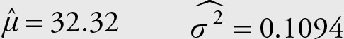
Since population variance is unknown we need to use
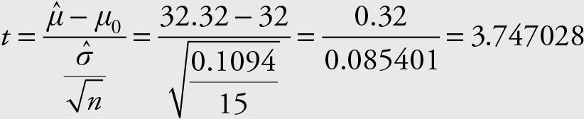
Using the following Excel command we obtain the exact P value.
= t.dist.rt(3.747028,14) = 0.001083
The probability of obtaining an average of $32.32, if the true population average is $32.00, is only 0.001083. This is a low probability. Therefore, we reject the null hypothesis in favor of the alternative hypothesis. Alternatively, we could say that the probability of type I error, if we reject the null hypothesis, is only 0.001083 and hence, we reject the null hypothesis. If you copy the value of the “t” into the formula for the P value you will get the same number as shown above, that is 0.001083. However, if you type in the rounded number, which is “3.74,” you would get “0.001098.” The first number is more accurate because it uses the precise answer for “t.”
Example 7.2
Test the claim that more than 50% of the stock prices for Microsoft close higher than $32.20. Use the sample from March 12 to March 30, 2012.
Solution
Sorting the data makes it easier to obtain the portion of sample prices over $32.20.
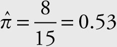
Based on the statement in the problem the alternative hypothesis is:
H1: π > 0.50 ⇒ H0: π = 0.5
From Table 7.2 the correct formula is:
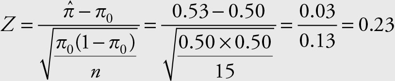
The probability of the region more extreme than Z = 0.23 is given by
P (Z > 0.23) = 0.5 – P (0 < Z < 0.23) = 0.5 – 0.0910 = 0.4090
Since the probability of type I error, if we reject the null hypothesis, is too high, we fail to reject the null hypothesis.
Example 7.3
Test the claim that the variance for the stock prices of Microsoft is greater than 0.9. Use the sample from March 12 to March 30, 2012.
Solution
Based on the statement in the problem the alternative hypothesis is:
H0: σ2 > 0.90 ⇒ H1: σ2 = 0.90
From Table 7.2 the appropriate formula is:
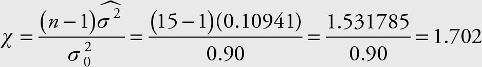
Using the following Excel command we obtain the P value:
= chisq.dist.rt(1.702,14) = 0.99997
Since the probability of type I error is too high, we fail to reject the null hypothesis.
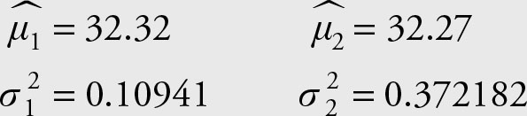
Example 7.4
Are the means for Microsoft stock prices for periods March 12–30 and April 2–21 the same?
Solution
The objective is to determine if μ1= μ2. Since this format is not of the form of a parameter equal to a constant, we rewrite the hypothesis as:
H0: μ1− μ2 = 0 H1: μ1− μ2 ≠ 0
Since no particular directional claim has been made, the test is a two-tailed test. The following information is available:
Since we do not know whether the variances are equal, we will test their equality first, that is,  Since this is of the form of a parameter equal to another parameter, it has to be modified to resemble a parameter = a constant format.
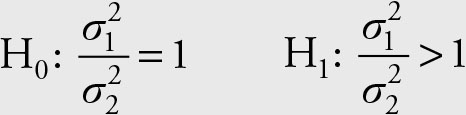
It is customary to express this alternative hypothesis in the “greater than one” format. To assure that the ratio of the sample variances is actually greater than one, always place the sample variance that is larger in the numerator.
From Table 7.2, the appropriate formula to test the equality of two variances is
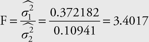
The P value for this statistic is obtained from the following Excel
command:
= f.dist.rt(3.4016,14,14) = 0.0144
Since the probability of type I error is low enough, we reject the null hypothesis that the two variances are equal. Therefore, from Table 7.2, the following test statistics is used for testing equality of the mean prices for the two periods.
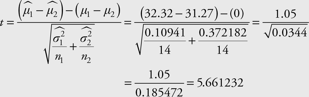
Using the following Excel command we obtain the exact P value.
= t.dist.rt(5.6612,28) = 0.000,002
Since the P value is low enough, we reject the null hypothesis that
the average prices of Microsoft stock are the same for the periods of March 12–30 and April 2–21.