
Some Applications of Descriptive Statistics
Introduction
The descriptive statistics that were covered in Chapters 1 and 2 provide summary statistics and graphical methods to present data in a more concise and meaningful way. Although those measures and methods are useful in their own right as demonstrated in the previous chapters, they are also used to further create more powerful statistical measures: some of which are discussed in this chapter. Later, in Chapter 7, these measures are utilized to provide statistical inference, which is the foundation for testing hypotheses in every branch of science.
Coefficient of Variation
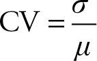
The coefficient of variation is the ratio of the standard deviation to the mean. In other words, the coefficient of variation expresses the standard deviation (the average error) as a percentage of the average of the population or sample. It is a relative measure of dispersion. It measures the standard deviation in terms of the mean.
 (3.1)
(3.1)
The coefficient of variation is independent of the units of measurement of the variables. If two populations have the same standard deviation, the one with the lower coefficient of variation has less variation.
Example 3.1
The manager of the mortgage department in a local bank has gathered the amounts for approved second mortgage loans for every 100th customer. The amounts are in dollars.
5,672 |
6,578 |
9,700 |
12,000 |
9,000 |
6,350 |
4,495 |
6,900 |
7,835 |
8,750 |
10,000 |
12,000 |
6,500 |
7,200 |
8,000 |
18,000 |
19,000 |
12,000 |
4,560 |
1,500 |
5,900 |
5,450 |
6,500 |
1,800 |
1,900 |
10,500 |
|
|
|
|
Calculate the coefficient of variation.
Solution
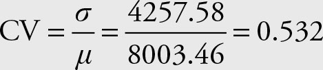
Coefficient of variation represents the average error as a fraction of the expected value. The coefficient of variation is useful in comparing data with different magnitudes. Assume that two stocks are rated similarly where they have the same characteristics such as objectives and the amount and frequency of dividends. In order to compare the relative variability of the average price of the two stocks, we use the coefficient of variation. Relative to the mean price, the stock with the lower coefficient of variation indicates lower variation and hence lower risk.
The coefficient of variation is also useful in the comparison of unrelated data, especially when the unit of measurement is different. For example, if the efficiency of a gas-powered lawn mower is compared to the reliability of an electric edger, then the machine with the lower coefficient of variation is more reliable.
The most effective use of the coefficient of variation is in the comparison of two different experiments by finding the ratios of their respective coefficients of variation, as is seen in the following example.
Example 3.2
Refer to the stock prices for Wal-Mart and Microsoft from Example 2.2. Determine which one is riskier using the data for March 2012.
Closing Prices of Wal-Mart (WMT) and Microsoft (MSFT) for the period from March 12 to March 30 and from April 2 to April 21, 2012
|
Date |
WMT |
MSFT |
Date |
WMT |
MSFT |
|
12 Mar. |
$60.68 |
$32.04 |
2 Apr. |
$61.36 |
$32.29 |
|
13 Mar. |
$61.00 |
$32.67 |
3 Apr. |
$60.65 |
$31.94 |
|
14 Mar. |
$61.08 |
$32.77 |
4 Apr. |
$60.26 |
$31.21 |
|
15 Mar. |
$61.23 |
$32.85 |
5 Apr. |
$60.67 |
$31.52 |
|
16 Mar. |
$60.84 |
$32.60 |
9 Apr. |
$60.13 |
$31.10 |
|
19 Mar. |
$60.74 |
$32.20 |
10 Apr. |
$59.93 |
$30.47 |
|
20 Mar. |
$60.60 |
$31.99 |
11 Apr. |
$59.80 |
$30.35 |
|
21 Mar. |
$60.56 |
$31.91 |
12 Apr. |
$60.14 |
$30.98 |
|
22 Mar. |
$60.65 |
$32.00 |
13 Apr. |
$59.77 |
$30.81 |
|
23 Mar. |
$60.75 |
$32.01 |
16 Apr. |
$60.58 |
$31.08 |
|
26 Mar. |
$61.20 |
$32.59 |
17 Apr. |
$61.87 |
$31.44 |
|
27 Mar. |
$61.09 |
$32.52 |
18 Apr. |
$62.06 |
$31.14 |
|
28 Mar. |
$61.19 |
$32.19 |
19 Apr. |
$61.75 |
$31.01 |
|
29 Mar. |
$60.82 |
$32.12 |
20 Apr. |
$62.45 |
$32.42 |
|
30 Mar. |
$61.20 |
$32.26 |
21 Apr. |
$59.54 |
$32.12 |
Solution
Let’s refer to Wal-Mart stock as “1” and to the Microsoft stock as “2.” Recall that we calculated the means and standard deviations for these stocks. The following information is available for the two stocks. Which one is relatively less risky and thus better?
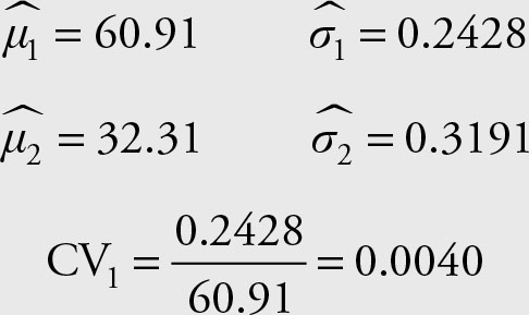

Therefore, stock 1, Wal-Mart, is less risky than stock 2, Microsoft.
Z Score
The Z score is a useful and intuitive concept and, as it will become evident, is used often in statistics. The Z score uses two of the more common parameters, the mean and the standard deviation. The problem of accurate and consistent measurement has been a difficult subject throughout history. The yardstick differed from one time to another and across different locations and cultures. Different countries and rulers tried to unify the unit of measurement. The closest unit to become universally accepted is the meter. Even the metric system is not commonly used in all quarters in spite of its ease and applicability. The metric system has its limitations too. One problem is the difference in scale. The following example demonstrates the problem.
County fairs have farming contests and they give prizes for the “best” in different categories. For example, the farmer with the biggest produce receives a prize. But by nature, even the largest apple on record is not a match for any pumpkin. Would it be fair to compare the amount of a cow’s milk with that of a goat? In economic terms, how can we compare the output of the most productive small manufacturer to that of a larger one, which is fully automated?
In statistics, everything is measured in relative terms. It makes no sense to compare the weight of a peach to that of a pumpkin, but comparing their relative weights makes perfect sense. Let’s have a peach that weighs 8.4 ounces and a pumpkin that weighs 274.9 ounces. Although the pumpkin is actually heavier, that might not be the case when other factors are considered. One factor is the average weight of peaches and pumpkins. A typical peach is about 6 ounces, while a typical pumpkin is 22 pounds, or 352 ounces. The peach in this example is somewhat heavier than an average peach while the pumpkin is actually lighter than an average pumpkin. Therefore, relatively speaking, the peach is heavier than the pumpkin. However, this is not enough. We also need to divide the distance from the mean for each produce by its typical or average error. Let’s assume that the standard deviation for peaches is 1.15 ounces. Therefore, the amount that the peach exceeds its average as measured by its own yardstick is (8.4 - 6) / 1.15 = 2.086 standard deviation. Let’s assume that the standard deviation for the pumpkin is 2.57 pounds or 16 × 2.57 = 41.12 ounces. Therefore, the pumpkin is (274.9 - 352) / 41.12 = -1.875 standard deviations below its expected weight. Therefore, the pumpkin is actually sub-par, while the peach is a prize winner. This is the essence of what is called a Z score and the procedure is known as standardization.
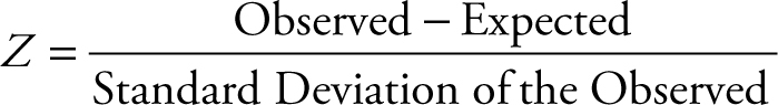
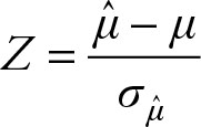
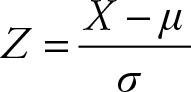
The Z score is defined as follows:
 (3.2)
(3.2)
 (3.3)
(3.3)
The expected value of an observation is its mean or (μ), its standard deviation is (σ). To obtain the Z score of an observed value, subtract its mean from its observed value and divide the result by the standard deviation of the observation.
The distance of an observation from its expected value is also called its error. Some of the different aspects of error will be discussed later in this chapter. The Z score is a scaled error. The unit of measurement of Z score is the standard deviation of the population or its sample estimate. Obtaining the Z score of an observation is also known as standardizing the value. The standardization process can be applied to any data or observation. If the item under consideration is a single observation from the population, the result is called the Z score.

Suppose two students are given the task of measuring the error of an observation. The first student found that the observation is 41.6666 feet. In fact, the decimal place is never-ending. Disliking decimal places and especially the never-ending ones, he measured the deviation of the data point from the mean in inches and was relieved to find out that it has no decimal place. He presented his error of the observation as 500 inches. The second student, using an electronic measuring “tape,” subtracted the observation from the mean and reported 0.007891414 miles as the error. While the first error seems large and the second seems small, both are the same. Note that 500 inches is 41.6666667 feet or 0.007891414 miles. Z score provides a unique and comparable measure of error to avoid the confusion that may arise from changes in units of measurement. Every error is reported in the units of its own standard deviation. Since the Z score is reported in terms of the standard deviation, it allows comparison of unrelated data measured in different units.
Z Score for a Sample Mean
If the value under consideration is the sample mean, ![]() , the resulting Z score would be:
, the resulting Z score would be:
 (3.4)
(3.4)
where ![]() is the sample mean, μ is its expected value, which is also the population mean, and the standard deviation of the sample is
is the sample mean, μ is its expected value, which is also the population mean, and the standard deviation of the sample is 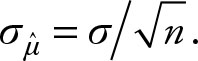 The standard deviation of the sample mean is also known as the standard error. In order to calculate the Z score for a sample mean, it is necessary to know the population variance. Usually, we do not know the population variance either. When the population variance is unknown, we must use a t value instead. We will discuss t distribution in more detail in Chapter 4. For the time being, we will assume that we know the population variance. The most realistic assumption is to use the sample variance as if it were the population variance.
Theorem 3.1 Chebyshev Theorem
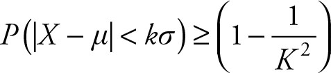
The proportion of observations falling within k standard deviations of the mean is at least
 (3.5)
(3.5)
This is the same Z score concept. The theorem indicates that we need to find the difference of a value from its mean, that is, (X - μ). Since the theorem applies to all the values within k standard deviations, that is, kσ on either side of the mean, the absolute value is desired. The theorem sets a minimum limit for the |X - μ| < kσ. Therefore, the Chebyshev theorem states that:
 (3.6)
(3.6)
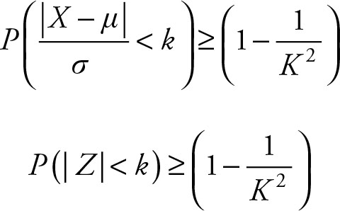
But since σ is a non-negative value, dividing both sides of the inequality |X - μ| < kσ by σ will not change the sign. Therefore,
 (3.7)
(3.7)
As is evident, the Z score is the core of the Chebyshev theorem. Chebyshev was one of the major contributors to the Central Limit Theorem, which will be discussed in Chapter 5.
The first part of the equation {P(|Z| < k)} is the same as the confidence interval of a range, which is covered in Chapter 6. The concept of Z score is also used in statistical inference, which is covered in Chapter 7.
Example 3.3
Determine what percentage of the Microsoft stock prices from March 12 to March 30, 2012, lay within the two standard deviations of their mean. Verify the correctness of the result by counting the prices that are within two standard deviations of the mean. Assume the population’s mean and variance are the same as the sample mean and variance, respectively. See Example 3.2 for data.
Solution
The sample mean and sample variance are given in Example 3.2 as:

Note that we are using the notation for population mean and population standard deviation to make sure that the theorem applies. The theorem requires the knowledge of population mean and standard deviation, and we are assuming them to be the values we obtained from the sample.
Insert the data in Equation 3.6:
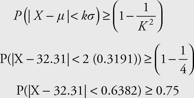
Therefore, at least 75% of the 15 observations will be within two standard deviations of the mean. Next we calculate the range “within 2 standard deviations.”
32.31 - 0.6382 = $31.67
32.31 + 0.6382 = $32.95
The easiest way to verify that the result is valid is to sort the data. You will notice that the lowest price is $31.91 and the highest price is $32.85. Therefore, 100% of the data are within two standard deviations of the mean, which exceeds the predicted minimal percentage of 75%.
Standardization
In order to be able to compare different objects with different scales we need a tool that places everything in a unified perspective. A value can be standardized by finding its distance from the population mean, that is, its individual error, and then scale the result or put it in perspective with respect to its standard deviation.
 (3.8)
(3.8)
The unit of measurement is in standard deviation.
If a data point is 72 and its expected value and standard deviation are 70 and 4.3, respectively, then the estimated error is ![]() Its standardized value is:
Its standardized value is:
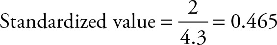
The data point is said to be 0.465 standard deviations to the right of its mean. If an ordinary data point is selected and its standardized value is calculated, then that value is called a Z score.
 (3.9)
(3.9)
Therefore, the two statements “the data point is 0.465 standard deviations above its mean” and “the Z score for the data point is 0.465” mean the same. Had the Z score been negative, then the data point would have been on the left side of its mean. If a random variable is from a population with known mean and variance, then its standardized value is called a Z score.
Example 3.4
Calculate the Z scores for closing prices of Microsoft stock from March 12 to March 30. Assume that the population’s mean and variance are equal to the sample mean and variance, respectively.
Solution
Use Equation 3.9 and the following values from Example 3.2:

Note that we are using the notation for population mean and population standard deviation to make sure that the theorem applies. The theorem requires the knowledge of population mean and standard deviation, and we are assuming that we know them to be the values we obtained from the sample.
|
Date |
MSFT |
Z Score |
|
12 Mar. |
$32.04 |
-0.86 |
|
13 Mar. |
$32.67 |
1.11 |
|
14 Mar. |
$32.77 |
1.43 |
|
15 Mar. |
$32.85 |
1.68 |
|
16 Mar. |
$32.60 |
0.89 |
|
19 Mar. |
$32.20 |
-0.36 |
|
20 Mar. |
$31.99 |
-1.02 |
|
21 Mar. |
$31.91 |
-1.27 |
|
22 Mar. |
$32.00 |
-0.99 |
|
23 Mar. |
$32.01 |
-0.95 |
|
26 Mar. |
$32.59 |
0.86 |
|
27 Mar. |
$32.52 |
0.64 |
|
28 Mar. |
$32.19 |
-0.39 |
|
29 Mar. |
$32.12 |
-0.61 |
|
30 Mar. |
$32.26 |
-0.17 |
|
0.00 |
The sum of the Z scores is provided at the bottom, which is zero. This is a mathematical property of individual errors, which add up to zero. See Definition 3.5.
Correlation Coefficient Is The Average of the Product of Z Scores
Correlation coefficient was introduced in Chapter 2. It measures the degree of association between two variables.
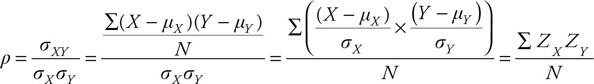
The above derivation depends on the definition of a parameter as a constant. This allows moving parameters, such as standard deviations, into a summation notation. Note that anything that is added and divided by the number of observations is an average number. In this case, the product of two Z scores (ZX ZY) is added and divided by N. Hence, correlation coefficient is the average of the product of two Z scores.
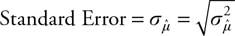
Standard Error
When data is obtained from a sample, the standard deviation of the estimated sample statistics is called a standard error. This concept will be addressed in detail when the sampling distribution of the sample mean is discussed in Chapter 5. As the distributional properties of sample standard deviation are different than that of the population standard deviation, we had to assume that the standard deviation obtained from the samples in Examples 3.2 and 3.4 were known to be the same as the population standard deviation.
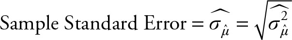
Usually, the standard deviation of the sample mean is also unknown and has to be estimated, which is represented with a hat.
Therefore, the correct representation of the t statistics from a sample is:
 (3.10)
Note that Equation 3.10 is called a t and not a Z as in Equation 3.4. The reason for the difference in names is due to the difference in the denominators of the two equations. Gosset1 showed that if the population variance is unknown and has to be estimated by the sample variance, then the resulting standardization does not have a normal distribution and does in fact have a student t distribution.
Definition 3.1
The Degree of Freedom is the number of elements that can be chosen freely in a sample. The degree of freedom only applies to a sample. The population parameters are constant values and are estimated by sample statistics.
Example 3.5
Let us have a small population, say, sized five. For example, consider a family with five children of ages 3, 5, 7, 8, and 9. Let us take samples without replacement of size three from this population. There will be 10 different possible samples. The population mean is 32/5 = 6.4, that is, the average age of the children is 6.4 years. The mean value governs the outcome of the average of the mean of the samples, as is demonstrated below. The 10 possible samples and their corresponding means are:
|
Sample |
Mean |
|
8, 3, 7 |
6 |
|
8, 3, 5 |
5.333 |
|
8, 3, 9 |
6.667 |
|
8, 7, 5 |
6.667 |
|
8, 7, 9 |
8 |
|
8, 5, 9 |
7.333 |
|
3, 7, 5 |
5 |
|
3, 7, 9 |
6.333 |
|
3, 5, 9 |
5.667 |
|
7. 5. 9 |
7 |
|
Total |
64 |
Even though none of the sample means equals the population mean, the population mean has exerted its influence on the sample means. Find the average of the 10 possible sample means. It is 64 / 10 = 6.4. Therefore, the expected value or the average of all the possible sample means is equal to the population mean. Even if we do not know the population mean, every population has a mean, and that mean will influence all the sample means. It is even possible to prove, mathematically, that the average of sample means is equal to the population mean. In mathematical statistics the average is formally defined as the expected value and is represented by an E, therefore, ![]()
In the Example 3.5, this means that any 9 of these 10 possible samples can be chosen freely. After 9 samples and their means are obtained, the 10th, or the last one, is forced to have a mean value such that the average of all the sample means equals the population mean. Let us assume that the fourth possible sample in the above list is the one that is not taken yet, and its mean has not been calculated. The mean of this sample has to be 64 - 57.222 = 6.778. Within this sample any two numbers can be selected at random, but the last one must be such a number that its average equals 6.778. Two of the three numbers 8, 7, and 5 can be randomly selected. Say 5 and 7 are selected. The last number must be 8, since this is the only number that will make the average of this sample equal to 6.778 and the average of all the sample means equal to m = 6.4. In general, n - 1 sample points can be selected at random, but the value of the remaining one will be determined automatically by the value of the population. One degree of freedom is lost for every parameter that is unknown and must be estimated by a statistics.
Computation of variance requires the knowledge of the population mean.
If the population mean μ is not known, the value of σ2 cannot be determined. If instead of μ its estimate is obtained, then the sample mean, or ![]() is used. The sample variance then is:
is used. The sample variance then is:
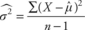
and it will lose one degree of freedom. The result of the adjustment to the sample variance—that is, dividing by the degree of freedom, n - 1, instead of the sample size, n—is that the sample variance becomes an unbiased estimate of the population variance.2
Properties of Estimators
Sample statistics are used as estimators of the population parameters. Since sample statistics provide a single value, they are also called point estimates. It is desirable to be able to compare different point estimates of the same parameters and provide useful properties.
Let θ, pronounced theta, be the population parameter of interest. Let its estimate be ![]() pronounced theta hat. Like any other point estimate,
pronounced theta hat. Like any other point estimate, ![]() is a sample statistic and a known variable.
is a sample statistic and a known variable.
Definition 3.2
If the expected value of a point estimate equals the population parameter, then the estimate is unbiased. In symbols:
 (3.11)
It can be shown that the sample mean (![]() ), variance
), variance  and proportion
 ![]() are all unbiased estimates of their corresponding population parameters.
are all unbiased estimates of their corresponding population parameters.
Definition 3.3
The efficiency of a point estimator is said to be higher if it has a smaller variance. If ![]() and
and ![]() are two point estimates of θ and Var
are two point estimates of θ and Var  then
then ![]() is more efficient than
is more efficient than ![]() . For example, the sample mean is more efficient than the sample median in estimating the population mean.
. For example, the sample mean is more efficient than the sample median in estimating the population mean.
Definition 3.4
A point estimate is a consistent estimator if its variance gets smaller as the sample size increases. The variance of the sample mean
will decrease as the sample size increases. As the sample size increases, the sample mean will have a smaller and smaller variance. And as it is an unbiased estimate of the population mean, it will get closer and closer to the population mean.
Error
Statistics deals with random phenomena. For a set of values X1, X2, ..., Xn there is a representative or expected value (mean). The Greek letter μ is used to represent the expected value. The difference of each value from the expected value, also called the deviation from the mean, represents an individual error.
Definition 3.5
An individual error is the difference between the value of an observation and its expected value. The expected value or the mean is the best estimate or representative of a population and, hence, the sample. For example, the average starting salary for an economics major in 2011 was $54,400. If a recent economics graduate is selected at random his or her expected income is $54,000 then the error associated with this observation is $400. In other words, the observation missed the expected value by $400. The reason for calling the deviation an error is that we do not have any explanation for the deviation other than a random error. Therefore, the error is what we cannot explain. Since observations vary at random, the errors vary at random as well. Furthermore, the portion that cannot be explained depends on the model or procedure used. Sometimes it is possible to explain part of variation of observations from their expected value by developing more sophisticated methods. The portions that can be explained by the new procedure are no longer “unexplained,” and, thus, not part of the error any more. The unexplainable portion is still called an error. Note that unless all the observations in a sample or population are identical, they will deviate from their expected value and, hence, have a random error.
Since there are as many individual errors as there are observations, we need to summarize them into fewer variables. A popular and useful statistic is the average or the mean. However, the average of individual errors is always zero because the sum of all errors is zero. Recall that individual errors are deviations from their expected values, some of which are negative and the others are positive. Thus, by definition, they cancel each other out and the sum of all deviations is always zero. Symmetric distributions have equal numbers of positive and negative individual errors, but this is not a necessary condition for their sum to add to zero. The sum of individual errors for non-symmetric distributions is also zero, in spite of the fact that the count of negative values is different from the count of the positive values. This is due to the fact that the expected value or the mean is the same as the center of gravity of the data. Imagine data on a line where they are arranged from smallest to largest. Placing a pin at the point of the average will balance the line.
There are several ways to overcome individual errors canceling each other out. One way is to use the absolute value of the individual errors. The average of the absolute values of the individual errors is called mean absolute error (MAE). The mean absolute error is commonly used in time series analysis. One advantage of MAE is that it has the same unit of measurement as the actual observations.
Another way to prevent individual errors from canceling each other out is to square them before averaging them. We are already familiar with this concept, which is called a variance.
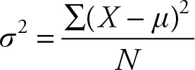
Definition 3.6
The variance is the average of the sum of the squared individual errors.
One advantage of variance over the mean absolute error is that it squares errors, which gives more power to values that are further away from the expected value. This makes the variances disproportionately large as individual errors get larger. The variances use of the squared values of the individual errors is its shortcoming as well because the unit of measurement for the variance is the square of the unit of measurement of the observations. If the observations are about length in feet, then the variance will be in feet squared, which is the unit of measurement of an area and not length. Seldom, if ever, the squared values of economic phenomenon have any meaning. If the variable of interest is price, measured in dollars, then the unit of measurement of its variance is in dollars-squared, which has no economic meaning. To remedy this problem, it is necessary to take the square root of variance.
Definition 3.7
The standard deviation is the square root of the variance.
Definition 3.8
The standard deviation is the average error.
How Close Is Close Enough?
If the sum of the residual is not zero, then check your formulas and computations. If the definitional formulas are used or the results are rounded off at early stages, the sum of individual errors may be different than zero. Use of computational formulas and less round-off will reduce or eliminate this problem provided the sample size is sufficiently large. If you use five decimal places, the final result can be accurate to about four decimal places. If you have been using five decimal places in your calculations and the sum of the residual is 0.00007, the property has not been violated. It is zero to four decimal places as expected.
Sum of Squares
The sum of squares of deviation of values from their expected value (mean) is a prominent component of statistics. As we saw previously, the square of these individual errors divided by the population size is called population variance. The concept is the same for a sample, except that the divisor is the degree of freedom. Earlier, it was explained that the portion of the phenomenon that cannot be explained is called an error, and that the variance is one way of representing it. When alternative models are used to explain part of the error, it is more meaningful to focus on the numerator alone, at least at first. The numerator, or variance, is also called total sum of squares (TSS). Once a set of data is collected then the TSS becomes fixed and will not change. The TSS will only change if another sample from the same population was collected at random. Decomposition of TSS is very common in a branch of statistics called experimental design. In experimental design methodology TSS is decomposed into different components based on the design. These components include treatment SS, block SS, main effect SS, and so forth. In all cases there is always a component that remains unexplained, and is referred to as residual or error SS. By definition, dividing this unexplained remainder by appropriate degrees of freedom would result in the variance of the experiment, customarily known as mean squared error (MSE) or mean squares error. As one would expect, the square root of MSE is called root MSE, which is the same as the standard error. Just as a reminder:
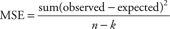
Note that the term in the parentheses is the individual error. The k in the denominator is the number of parameters in the model, and the entire denominator is the degrees of freedom.
Skewness
As you noticed in Chapter 2, several of the relationships between mean, mode, and median were described. The relationship between these parameters can also be used to determine if the data are symmetric and the extent of the pointedness of the data. Of course, the data cannot be flat, pointed, symmetric, or skewed. The fact is that we are talking about the shapes of data when they are plotted.
Definition 3.9
The skewness refers to the extent that a graph of a distribution function deviates from symmetry. A distribution function that is not symmetric is either negatively skewed, as in Figure 3.1, or positively skewed, as in Figure 3.2.
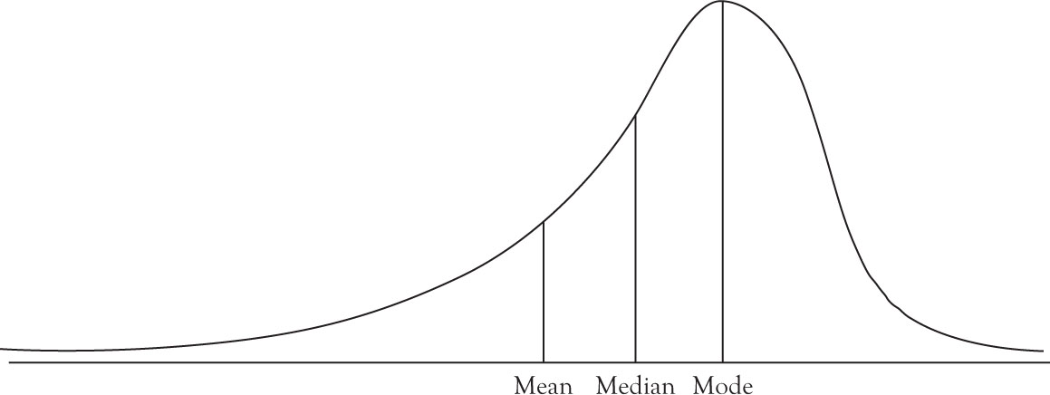
Figure 3.1. Negatively skewed distribution.
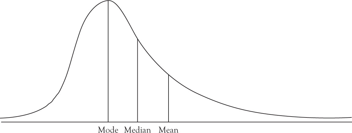
Figure 3.2. Positively skewed distribution.
Relation Between Mean, Median, and Mode
The mean, median, and mode of symmetrical distributions are identical. If the distribution is positively skewed, the order of magnitude is
Mode < Median < Mean(3.12)
If the distribution is negatively skewed, the order of magnitude is
Mean < Median < Mode(3.13)
The importance of skewness is in its use to test if the data follows a normal distribution. Normal distribution function is discussed in Chapter 4.
Definition 3.10
The Pearson coefficient of skewness is defined as:
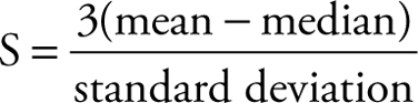
The range of skewness is -3 < S < 3, and for a symmetric distribution S = 0. The sign of the Pearson coefficient of skewness determines if it is positively or negatively skewed.
Definition 3.11
Kurtosis is a measure of pointedness or flatness of a symmetric distribution. The exact definition of Kurtosis requires the knowledge of the moments, which is beyond the scope of this text. A positive Kurtosis indicates the distribution is more pointed than the normal distribution, and a negative value for Kurtosis indicates the distribution is flatter than normal distribution. Kurtosis and skewness are commonly used to test whether a data set follows a normal distribution.