
Sampling Distribution of Sample Statistics
Sampling
A sample is a subset of population that is collected in a variety of ways. The process of collecting samples is called sampling. As will become evident in this chapter, random sampling is very important for establishing the necessary theories for statistical analysis. For example, if a firm has 500 employees and 300 of them are men, then the probability of choosing a male worker at random is 300/500 = 0.60 or 60%. Sampling techniques are not limited to random sampling. Each sampling technique has its advantages and disadvantages. This text is not going to focus on various sampling techniques. After a brief discussion about sampling, the focus will be on the properties and advantages of random sampling. Theories that are necessary for performing statistical inferences and are related to sampling are discussed in this chapter. In Chapter 2, we explained statistics and defined it as:
Statistics is a numeric fact or summary obtained from a sample. It is always known, because it is calculated by the researcher, and it is a variable. Usually, statistics is used to make an inference about the corresponding population parameter.
The only way to know the parameters of a population is to conduct a census. Conducting a census is expensive and, contrary to common belief, is not always accurate. Since a census takes time, it is possible that the findings are already inaccurate by the time the massive information is obtained and verified for mistakes and tabulated. On average, it takes about 2 years or more to release the census results in the United States. During this time, all variables of collected data change; for example, new babies are born, some people die, and others move. Sampling, on the other hand, can be performed in a shorter amount of time, while occasionally the census information is sampled in order to release some of the results quicker.
Sometimes, taking a census is not an option. This is not only due to the time and money involved, but also because the census itself might be destructive. For example, in order to find out the average life of light bulbs, they must be turned on and left until they burn out. Barring mistakes, this would provide the average life of the light bulbs, but then there will not be any light bulbs left. Similarly, determining if oranges were not destroyed by frost requires cutting them up. Other examples abound. Conversely, there are lots of other reasons where it is unrealistic, if not impossible, to conduct a census to obtain information about a population and its parameters.
Collecting sample data is neither inexpensive nor effortless. Sampling textbooks devote many pages of explanation on how to obtain random samples from a population. One simple, but not necessarily pragmatic or efficient way, is to assign ID numbers to all members of the population. Then pull the desired number of sample points by drawing lots at random of the ID numbers.
In this instance, our interest in sampling is very limited. We are interested in obtaining an estimate from a relatively small portion of a population to obtain insight about its parameter. The knowledge of parameters allows meaningful analysis of the nature of the characteristics of interest in the population and is vital for making decisions about the population of the study.
As discussed earlier, summary values obtained from a sample are called statistics. Since statistics are variables, different samples result in slightly different outcomes and the values of statistics differ, which is the consequence of being a random variable. It is possible to have many samples and thus many sample statistics, for example, a mean. It turns out that the sample means have certain properties that are very useful. These properties allow us to conduct statistical inference.
Definition 5.1
Statistical inference is the method of using sample statistics to make conclusions about a population parameter.
Statistical inference requires the population of interest to be defined clearly and exclusively. Furthermore, the sample must be random in order to allow every member of the population an equal chance to appear in the sample, and to be able to take advantage of statistical theories and methods. Later, we will cover the theories that demonstrate why random sampling provides sufficient justification for making inferences about population parameters.
The method of using information from a sample to make inference about a population is called inductive statistics. In inductive statistics, we observe specifics to make an inference about the general population. This chapter introduces the necessary theories, while the remaining chapters provide specific methods for making inferences under different situations. We also use deductive methods in statistics. In deductive methods, we start from the general and make assertions about the specific.
Statistical inference makes probabilistic statements about the expected outcome. It is essential to realize that since random events occur probabilistically, there is no “certain” or “definite” statement about the outcome. Therefore, it is essential to provide the probability of the outcome associated with the expected outcome.
Sample Size
Before we discuss the role of randomness and the usefulness or effectiveness of a sample, it is important to understand how other factors influence the effectiveness of the sample statistics by providing reliable inference about a population parameter. Even if a sample is chosen at random, two other factors attribute to the reliability of the sample statistics. They are the variance of the population and the sample size. For a population with identical members, the necessary sample size is one. For example, if the output of a firm is always the same, say 500 units per day, then choosing any single given day at random would be sufficient to determine the firm’s output. Note that in the previous example, there was no need to sample at random, although one can argue that any day that is chosen is a random day. However, if the output changes every day due to random factors such as sickness, mistakes during production, or breakdown of equipment, then sample size must increase. It is important to understand the possible difference in output among the days of the week and the month, if applicable. For example, Mondays and Fridays might have lower output. By Friday, workers might be tired and not as productive. Machinery might break or need to be cleaned more often towards the end of the week. On Mondays, workers might be sluggish and cannot perform up to their potential. Workers might be preoccupied towards the end of the month or early in the month when they are running out of money, or when their bills are due. These are just some of the issues that might have to be considered when setting up sampling techniques in order to assure the randomness of the sampled units. Therefore, there should be a direct relationship between the sample size and the variance of the population, and larger samples must be taken from populations with larger variance. Since statistical inference is probabilistic to obtain higher levels of confidence, we should take larger samples.
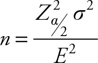
It can be shown that the required sample size for estimating a mean is given by:
 (5.1)
(5.1)
where,  is the square of the Z score for desired level of significance,
σ2 is the variance of the population,
E2 is the square of tolerable level of error.
Example 5.1
Assume that the population’s standard deviation for the output level is 29. Also, assume that we desire to limit our error to 5%, which makes the level of significance 95%. Let’s allow the tolerable level of error to be 5.
To obtain the sample size, we first need to obtain the Z score. In Figure 5.1, the area in the middle is 95%. Therefore, the area at the two tails is equal to 0.05.
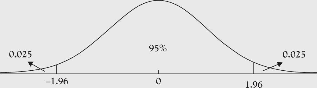
Figure 5.1. Graph of a normal distribution.
Furthermore, the area between zero and the right-hand cutoff point is 0.45, which according to the table corresponds with a Z score of 1.96. In Excel, you could use the following formula:
=NORMINV (0.975,0,1)
Note that the answer from Excel is 1.959964, which is slightly off.
The necessary sample size is given by:
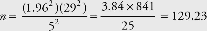
Since fractional samples are not possible, we must always use the next integer to assure the desired level of accuracy. Therefore, the minimum sample size should be 130.
Definition 5.2
The reliability of a sample mean (![]() ) is equal to the probability that the deviation of the sample mean from the population mean is within the tolerable level of error (E):
) is equal to the probability that the deviation of the sample mean from the population mean is within the tolerable level of error (E):
![]() (5.2)
(5.2)
Example 5.2
A 95% reliability for the sample mean is given by the area between the two vertical lines in Figure 5.2.
![]()
And the tolerable level of error is equal to:
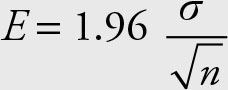
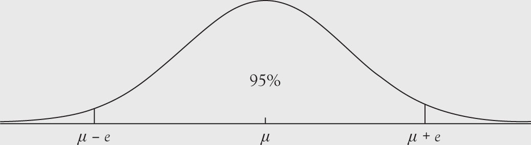
Figure 5.2. The range for 95% reliability for sample mean.
An astute student will notice that in order to estimate the sample size, it is necessary to know the variance. It is also imperative to understand that in order to calculate variance, one needs the mean, which apparently, is not available; otherwise we would not have to estimate it. Sometimes one might have enough evidence to believe that the variance for a population has not changed, while its mean has shifted. For example, everybody in a country is heavier, but the spread of the weights is no different than those in the past. In situations that the known variance is also believed to have changed, the only solution is to take a pre-sample to have a rough idea about the mean and variance of the population and then use sample estimates as a starting point to determine a more reliable sample size.
Sampling Distribution of Statistics
As stated earlier, sample statistics are a random variable and change from sample to sample. This means that the actual observed statistics is only one outcome of all the possible outcomes. A sampling distribution of any statistics explains how the statistics differ from one sample to another. The most commonly used statistics are sample mean and sample variance. Therefore, we will study their sampling distributions by approaching this subject in a systematic way. We begin with sampling distribution for one sample mean and distinguish between the cases when population variance is known and when it is unknown. Next, we introduce two sample means and address the cases of known and unknown variances, and so on. However, before embarking on this mission, it is necessary to discuss the Law of Large Numbers and the Central Limit Theorem, which are the foundations of inferential statistics.
Theorem 5.1 Law of Large Numbers
For a sequence of independent and identically distributed random variables, each with mean (μ) and variance (σ2), the probability that the difference between the sample mean and population mean is greater than an arbitrary small number will approach zero as the number of samples approaches infinity.
The theorem indicates that as the number of random samples increase, the average of their means approaches the population’s mean. Since sample means are statistics and random, their values change and none of them is necessarily equal to the population mean. The law of large numbers is essential for the Central Limit Theorem.
Theorem 5.2 Central Limit Theorem
Let θ be a population parameter. Let ![]() be the estimated value of q that is obtained from a sample. If we repeatedly sample at random from this population, the variable
be the estimated value of q that is obtained from a sample. If we repeatedly sample at random from this population, the variable ![]() will have the following properties:
will have the following properties:
1.The distribution function of ![]() can be approximated by normal distribution
can be approximated by normal distribution
2.E (![]() ) = q
) = q
3. 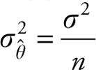
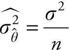
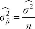
Property number 2, above, states that the expected value of the sample statistics (![]() ) will be equal to the population parameter (θ). In other words, the average of all such sample statistics will equal the actual value of the population parameter. Note that as the sample size increases, the sample variance of the estimate
) will be equal to the population parameter (θ). In other words, the average of all such sample statistics will equal the actual value of the population parameter. Note that as the sample size increases, the sample variance of the estimate  decreases. Therefore, as the sample size increases, the sample statistics (estimate) gets closer and closer to the population parameter (θ).
The approximation improves when the sample size is large and the population variance is known. When the population variance is unknown and the sample size is small, then the sample statistics ![]() will have the following properties:
will have the following properties:
1.The distribution function of ![]() can be approximated by t distribution with (n - 1) degrees of freedom
can be approximated by t distribution with (n - 1) degrees of freedom
2.E(![]() ) = θ
) = θ
3.  .
.
As the sample size increases, the distinction between normal distribution and t distribution vanishes.
The general population parameter θ can be the mean (μ), the proportion (π), or the variance (σ2). For each of the above three parameters, we may be dealing with one or two populations (comparison). In each case, the mean and variance of the estimator will be different. There will be 10 different cases, which can be viewed in a summary table.
Lemma 5.1
Let Y = X1 + X2 + … + Xn, where the Xs are random variables with a finite mean (μ) and a finite and known positive variance (σ2). Then,
has a standard normal distribution, which indicates that it is a normal distribution with mean = 0 and variance = 1.
Sampling Distribution of One Sample Mean
Population Variance Is Known
Sample mean is a statistics. Assume we know the variance of a population from which the sample mean is obtained. Let (![]() ) be the mean of a random sample of size n from a distribution with a finite mean (μ) and a finite and known positive variance (σ2). Using the central limit theorem, we know the following is true about the sample mean (
) be the mean of a random sample of size n from a distribution with a finite mean (μ) and a finite and known positive variance (σ2). Using the central limit theorem, we know the following is true about the sample mean (![]() ):
):
1.The distribution function for (![]() ) can be approximated by the normal distribution (since the population variance is known)
) can be approximated by the normal distribution (since the population variance is known)
2.E(![]() ) = μ
) = μ
3.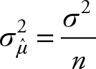
Therefore, we can use the normal table values for comparison of the standardized values of the sample mean. The knowledge of population variance σ2 is essential for completion of the third outcome. The distribution function of sample mean for samples of size 30 will be close to normal distribution. For random variables from a population that is symmetric, unimodal, and of the continuous type, a sample of size 4 or 5 might result in a very close approximation to normal distribution. If the population is approximately normal, then the sample mean would have a normal distribution when sample size is as little as 2 or 3.
Example 5.3
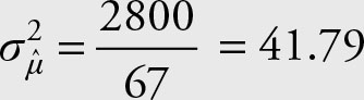
Assume that the variance for daily production of a good is 2800 pounds. Find the sampling distribution of the sample mean ![]() for a sample of size 67.
for a sample of size 67.
Solution
1.The sampling distribution of sample mean ![]() is normal
is normal
2.E( ^ ) = μ
3.
As we see, there is very little computation involved. Nevertheless, the theoretical application is tremendous.
Example 5.4
Assume that the variance for daily production of a good is 2800 pounds. What is the probability that in a sample of 67 randomly selected days the output is 15 pounds, or more, below average?
Solution
We are interested in a deviation from the population average.
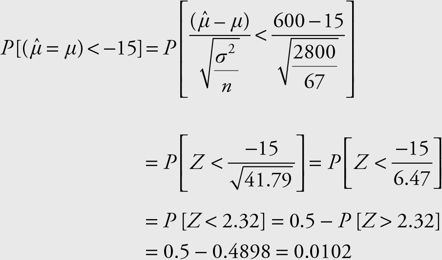
Note that for this problem, we do not need to know the true population mean since we are interested in knowing the probability of producing below the population mean.
Population Variance Is Unknown
Let (![]() ) be the mean of a random sample of size n from a distribution with a finite mean and a finite and unknown positive variance (σ2). According to the Central Limit Theorem:
) be the mean of a random sample of size n from a distribution with a finite mean and a finite and unknown positive variance (σ2). According to the Central Limit Theorem:
1.The distribution of (![]() ) can be approximated by a t distribution function
) can be approximated by a t distribution function
2.E(![]() ) = μ
) = μ
3.
Therefore, we can use the t table values, which are provided in the Appendix for comparison of the standardized values of the sample mean.
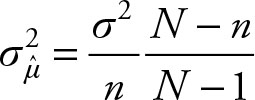
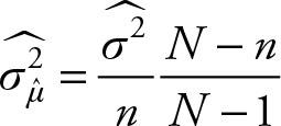
When the population size is small, or if the sample size to population size n/N is greater than 5%, you should use a correction factor with the variance. The correction factor is N – n/N – 1. For finite populations, the variance of the sample mean becomes:
 known variance
 unknown variance
Summary
Distribution function for one sample mean
|
Distribution |
Mean |
Variance |
|
|
Population Variance is known |
Normal |
μ |
|
|
Population Variance is unknown |
t |
μ |
|
Sampling Distribution of One Sample Proportion
Let ![]() be a proportion from a random sample of size n from a distribution with a finite proportion (π) and a finite positive variance (σ2). When both nπ ≥ 5 and n(1 - π) ≥ 5, then the following theorem is correct based on the Central Limit Theorem:
be a proportion from a random sample of size n from a distribution with a finite proportion (π) and a finite positive variance (σ2). When both nπ ≥ 5 and n(1 - π) ≥ 5, then the following theorem is correct based on the Central Limit Theorem:
1.The distribution of ![]() can be approximated by a normal distribution function
can be approximated by a normal distribution function
2.E ![]() = π
= π
3.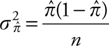
Note that in order to obtain the variance of the sample proportion, we must estimate the population proportion using the sample proportion. Thus, 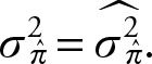
Therefore, we can use the normal table values for comparison of the standardized values of the sample mean. Note that the symbol pi (π) is used to represent the sample proportion and has nothing to do with π = 3.141593…
An added advantage of using sampling distribution of sample proportion is that you can use normal approximation to estimate probability of outcome for binomial distribution function without direct computation or the use of binomial distribution tables. When both n π ≥ 5 and n(1 - π) ≥ 5 it is reasonable to approximate a binomial distribution using a normal distribution.
Sampling Distribution of Two Sample Means
The extension from the distribution function of a single sample mean to two or more means is simple and follows naturally. However, it is necessary to introduce appropriate theories.
Theorem 5.3 The Expected Value of Sum of Random Variables
Let Y = X1 + X2 + … + Xn, where the Xs are random variables. The expected value of Y is equal to the sum of the expected values of Xs.
E(Y ) = E(X1) + E(X2) + … + E(Xn)
Theorem 5.3 does not require that Xs be independent. This theorem allows us to sum two or more random variables.
Sampling Distribution of Difference of Two Means
When conducting inferences about two population parameters, there are two sample statistics, one from each population. Often, in order to conduct an inference the relationship between the parameters, and hence the corresponding statistics, has to be modified and written as either the difference of the parameters or the ratio of the parameters. This requires knowledge of the distribution function for the difference of two sample statistics or the distribution function for the ratio of two sample statistics. In this section, the sampling distribution of the difference of two sample means is discussed. Choose a distribution function for the difference of two sample proportion or the distribution function for the ratio of two variances to access those distribution functions. This section will address the distribution function of the difference of two means.
The Two Sample Variances Are Known and Unequal
Let  be the means of two random samples of sizes n1 and n2 from distributions with finite means μ1 and μ2 and finite positive known and unequal variances
  Let n1 and n2 be the respective sample sizes. According to the Central Limit Theorem and Theorem 5.3:
1.The distribution of  is normal
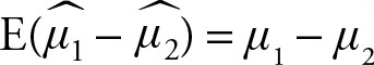
2. 
3.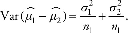
Note that the variances of the two samples are added together, while the means are subtracted. Therefore, we can use the normal table values for comparison of the standardized values of the differences of sample means.
The Two Sample Variances Are Known and Equal
Let be the means of two random samples of sizes n1 and n2 from distributions with finite means μ1 and μ2 and finite positive known and equal variances Let n1 and n2 be the respective sample sizes. According to the Central Limit Theorem and Theorem 5.3:
1.The distribution of is normal
2.
3.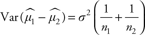
Since 
The Two Sample Variances Are Unknown and Unequal
Let be the means of two random samples of sizes n1 and n2 from distributions with finite means μ1 and μ2 and finite positive unknown and unequal variances Let n1 and n2 be the respective sample sizes. According to the Central Limit Theorem and Theorem 5.3:
1.The distribution of is normal
2.
3.
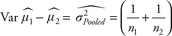
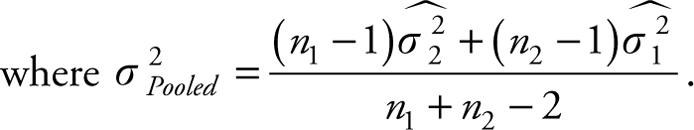
The Two Sample Variances Are Unknown and Equal
Let be the means of two random samples of sizes n1 and n2 from distributions with finite means μ1 and μ2 and finite positive unknown and equal variances Let n1 and n2 be the respective sample sizes. According to the Central Limit Theorem and Theorem 5.3:
1.The distribution of  is normal
2. 
3. 
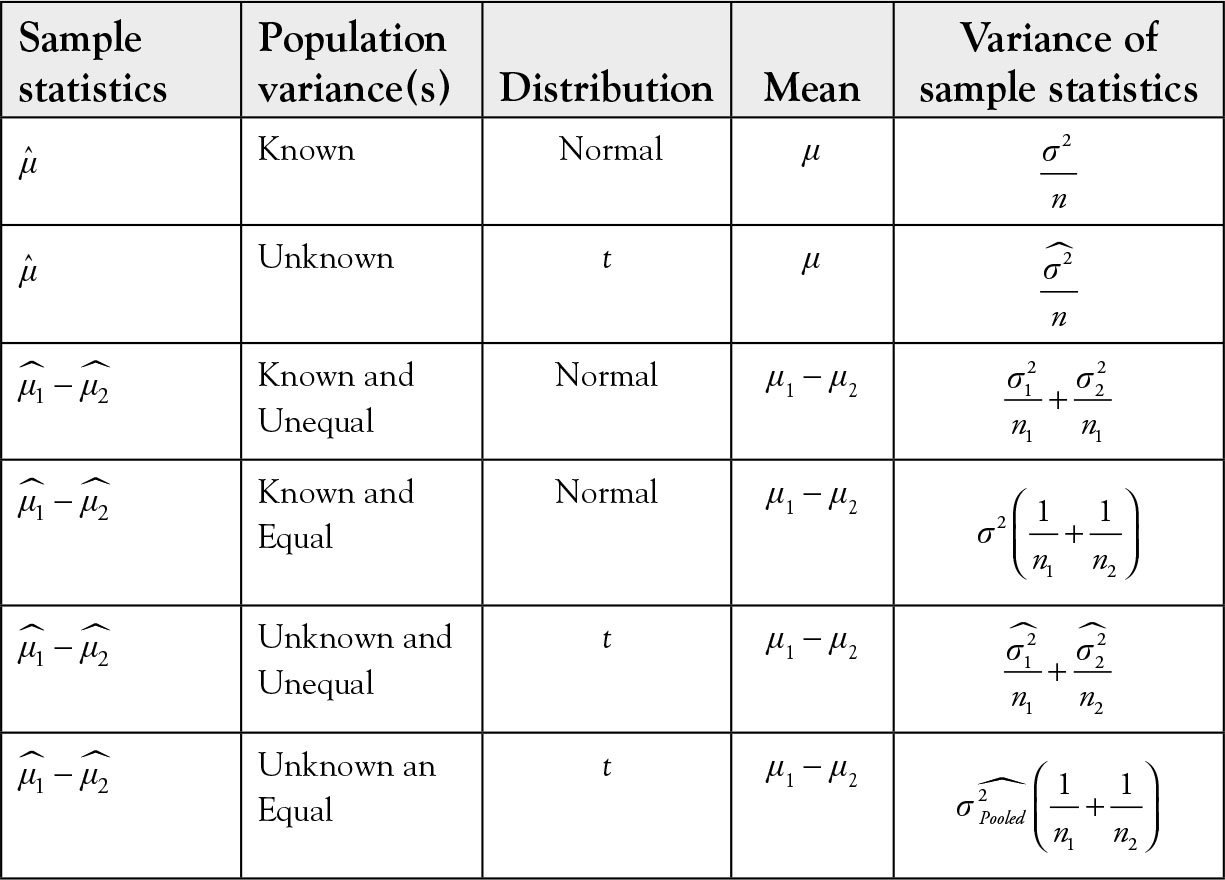
Summary of Sampling Distribution of Sample Means
Do not let these seemingly different and possibly difficult formulae confuse you. They are similar. The most common case is case 3, which is listed earlier. The first three cases can use this formula without any problem. The last case, earlier, takes advantage of the fact that there are two estimates of the unknown variance instead of one. Logic dictates that it would be better to average the two estimates using their respective sample sizes as weights. Table 5.1 provides a summary of sample statistics, its distribution functions, and its parameters for one and two sample means.
Table 5.1 Summary of Sampling Distribution for Sample Mean
Sampling Distribution of Difference of Two Proportions
When conducting inferences about two population parameters there are two sample statistics, one from each population. Often, in order to conduct an inference, the relationship between the parameters, and hence the corresponding statistics, has to be modified and written as either the difference of the parameters or the ratio of the parameters. This requires knowledge of the distribution function for the difference of two sample statistics or the distribution function of the ratio of two sample statistics. In this section, sampling distribution of the difference of two sample proportions is discussed. Choose the distribution function for the difference of two means or the distribution function for the ratio of two variances to access distribution functions for differences of two means or the ratio of two variances. This section will address the distribution function of the difference of two proportions.
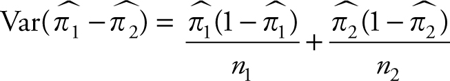
Let  be the proportions of interest in two random samples of sizes n1 and n2 from distributions with finite proportions π1 and π2 and finite positive variances According to the Central Limit Theorem:
1.The distribution of  is normal
2. 
3. 
Therefore, we can use the normal table values for comparison of the standardized values of the sample mean.
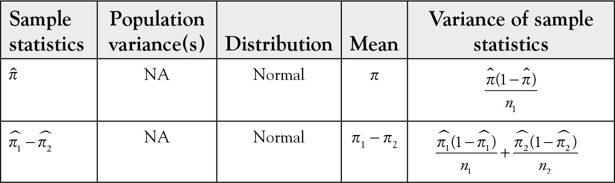
In practice, π1 - π2 is not known and their estimates, respectively, are used in calculating the variance of . The distribution function, expected value, and standard deviation for one and two sample proportions are given in Table 5.2.
Sampling Distribution of Sample Variance
Theorem 5.4
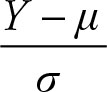
Let the random variable X have normal distribution with mean μ and variance σ2, then random variable
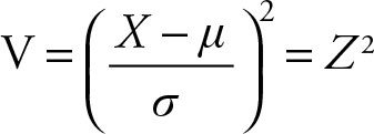
has a chi-squared distribution with one (1) degree of freedom, which is shown as χ2(1). Z is the same Z score as discussed in previous chapters, which consists of individual error divided by average error.
Chi-squared distributions are cumulative. Therefore, when n chi-squared distribution functions are added up, the result is another chi-squared distribution with n (sum of n distribution functions each with one) degree of freedom.
Theorem 5.5
Let random variables X1, X2, …, Xn have normal distribution each with mean μ and variance σ2 then the sum 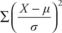 has a chi-squared distribution with n degrees of freedom. From this relation, we can build confidence intervals for one and two variances, and test hypothesis for one and two variances.
Sampling Distribution of Two Samples Variances
When conducting inferences about two population parameters, there are two sample statistics, one from each population. Often, in order to conduct an inference, the relationship between the parameters, and hence the corresponding statistics, has to be modified and written as either the difference of the parameters or the ratio of the parameters. This requires knowledge of the distribution function of the difference of two sample statistics or the distribution function of the ratio of two sample statistics. In this section, the sampling distribution of the ratio of two sample variances is discussed. Choose the distribution function for difference of two means or the distribution function for difference of two proportions to access distribution functions for differences of means or proportions. This section will address the distribution function of the ratio of two variances.
Theorem 5.6
Let random variables X1, X2, …, Xm have normal distribution each with mean μ1 and variance ![]() and the random variable Y1, Y2, …, Yn have normal distribution each with mean μ2 and variance
and the random variable Y1, Y2, …, Yn have normal distribution each with mean μ2 and variance ![]() then random variable
then random variable
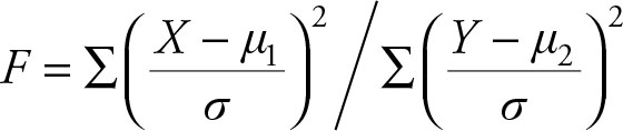
has an F distribution with m and n degrees of freedom.
Note that in Theorem 5.6, we could have expressed the numerator and denominator in terms of the corresponding chi-square distributions as stated in Theorem 5.5, which in turn is built upon Theorem 5.4.
In practice, when populations are not known, they are substituted by their respective sample variances.
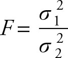
It is assumed that the variance labeled ![]() is greater than the variance labeled
is greater than the variance labeled ![]() . Tabulated values of F are greater than or equal to 1.
. Tabulated values of F are greater than or equal to 1.
The most common use of F distribution at this level is for the test of hypothesis of equality of two variances. This test provides a way of determining whether or not to pool variances when testing for the equality of two means with unknown population variances. First, test the equality of variances. If the hypothesis is rejected, then the variances are different and are not pooled. If the hypothesis is not rejected, then the variances are the same and must be pooled to obtain a weighted average of the two estimated values
Another use of F distribution is in testing three or more means. When testing a hypothesis that involves more than two means, we cannot use the t distribution. Test of hypothesis and the use of t and F distributions are discussed in Chapter 6.
Efficiency Comparison Between Mean and Median
Let ![]() be the sample mean and
be the sample mean and ![]() be the sample median. The expected value of, both, sample mean and sample median is equal to population mean. That is, both provide unbiased estimates of the population mean. However, as shown below, the sample mean is more efficient than the sample median in estimating the population mean. An estimator of a parameter is said to be more efficient than another estimator if the former has smaller variance. According to Central Limit Theorem, the variance of the sample mean (
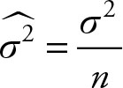
be the sample median. The expected value of, both, sample mean and sample median is equal to population mean. That is, both provide unbiased estimates of the population mean. However, as shown below, the sample mean is more efficient than the sample median in estimating the population mean. An estimator of a parameter is said to be more efficient than another estimator if the former has smaller variance. According to Central Limit Theorem, the variance of the sample mean (![]() ) is
) is
It can be shown that the variance of the median is
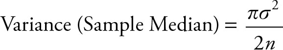
where π = 3.141593…
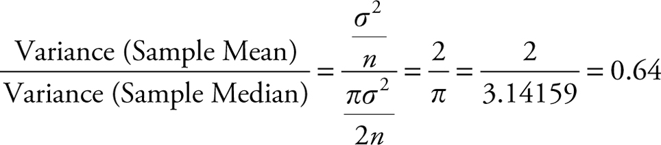
Therefore, ![]() is more efficient than median in estimating the population mean. The variance of the sample median from a sample of size 100 is about the same as the variance of the sample mean from a sample of size 64.
is more efficient than median in estimating the population mean. The variance of the sample median from a sample of size 100 is about the same as the variance of the sample mean from a sample of size 64.
It is worthwhile to note the following discrepancy, which is caused by having a different orientation or starting point.
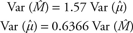
Therefore, the variance of sample mean is only 64% of the variance of the sample median. In estimating population mean, if we take a sample of size 100 and use the sample mean as the estimator, we will get a certain variance and hence, an error. To obtain the same level of error using the sample median to estimate the population mean, we need a sample of 157, which is 1.57 times more than 100.
Recall that when extreme observations exist, sample median is preferred to sample mean because it is not influenced by extreme values. For example, in real estate it is of interest to know the price of a typical house. The industry reports the prices of homes listed, sold, or withdrawn from the market each month. Usually, only a small fraction of existing homes is listed, sold, or withdrawn from the market. This causes large fluctuations in the average prices of these groups. The industry reports the median instead of the average price for the listings. Both sample mean and sample median are unbiased estimates of population mean, however, the latter is not influenced by the extreme high or low prices and thus is a better short-run estimator. Since sample median is less efficient than sample mean in estimating the population mean, larger samples are needed.