
Numerical Descriptive Statistics for Quantitative Variables
Introduction
One of the purposes of descriptive statistics is to summarize the information in the data for a variable into as few parameters as possible. Measures of central tendency provide concise meaningful summaries of the population. Measures of central tendency are addressed in the below section. However, measures of central tendency are often not enough to provide the full picture. The addition of measures of dispersion provides a more complete picture. Measures of dispersion are covered in next, followed by measures of association.
Measures of Central Tendency
Mean
The arithmetic mean, or simply the mean, is the most commonly used descriptive measure. Other names for the mean are average, mathematical expectation, and the expected value. This section deals with raw or ungrouped data.
Arithmetic Mean
The mean takes the concept of condensing information to the extreme. The mean, a single value, is the representative or typical value that represents a population. The mean is also known as the average, and more formally as the expected value. The mean is the sum of all the elements in the population divided by the number of the elements.
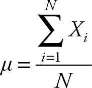 (2.1)
(2.1)
where μ, pronounced mu, is the symbol used to represent the mean; S, pronounced sigma, represents the sum of some random variables. When there is no ambiguity, we can simply write:
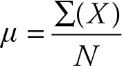 (2.2)
(2.2)
The mean is a parameter and provides information about the central tendency of the population. The mean is the representative, or expected value, of the population. For example, when we say that the average income of a country is $45,000, we are stating that if a person is selected at random his income is expected to be around $45,000. The mean is the expected value or the typical representative of a population when there is no other information.
The mean, though being the most widely used and most important parameter of the population, has its limits. It is susceptible to extreme values. Since all values of the population are used in calculation of the mean, a single very large or very small value can have a major impact on it. This is not quite as important in the case of the population as it is with samples.
Sample Mean
The sample mean is the sum of the sample values divided by the sample size.
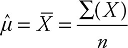 (2.3)
(2.3)
Note that we used both, ![]() pronounced mu-hat, and
pronounced mu-hat, and ![]() pronounced x-bar to represent the sample mean. Both are widely accepted. However,
pronounced x-bar to represent the sample mean. Both are widely accepted. However, ![]() has several advantages over
has several advantages over ![]() The first advantage is that it reduces the number of symbols that one has to learn in half. The population parameter is μ and its estimate μ. The second advantage is that it takes the guesswork out of which statistics you are dealing with, as long as you remember the population parameter. The third advantage is that it provides a reasonably simple rule to follow. Population parameters are represented by Greek letters, and sample statistics are represented by Greek letters with a hat on them.
The first advantage is that it reduces the number of symbols that one has to learn in half. The population parameter is μ and its estimate μ. The second advantage is that it takes the guesswork out of which statistics you are dealing with, as long as you remember the population parameter. The third advantage is that it provides a reasonably simple rule to follow. Population parameters are represented by Greek letters, and sample statistics are represented by Greek letters with a hat on them.
Definition 2.1
Statistics is a numeric fact or summary obtained from a sample. It is always known, because it is calculated by the researcher and it is a variable. Statistics is also used to make inferences about the corresponding population parameter.
The sample mean is a statistic. It is used to estimate the population parameter μ.
Example 2.1
An anthropologist is studying a small community of gold miners in a remote area. The community consists of nine families. The family income is reported below in thousands of dollars. Find the sample mean. This data is hypothetical, but plausible. We use this data to show computational detail.
66, 58, 71, 73, 64, 70, 66, 55, 75
Solution
A careful reader would remember that the same data and scenario was introduced in Example 1.4 but with a major difference. The data there was presented as population data. The idea of a small community with nine families is acceptable but a sample of nine is more plausible. We are using the same data for ease of computation and we limit the data size to avoid tedious computations. Nevertheless, we use actual data with more observations in different parts of the texts as well.
The sample mean is:

The expected income (in thousands of dollars) of any family from this population is 66.444. This statistic is an estimate of the population parameter μ.
We did not provide an example for the population mean because most populations are large and it would take a lot of space to display such a vast amount of data. In addition, we were concerned that you would not see the forest for the trees. The procedure is nevertheless the same. We can assume that the above data is actually the population and obtain the mean, which would be the same number. However, there is a major difference between the sample mean and population mean, as between any statistics and parameter. The former is a variable while the latter is a constant. In actual research we seldom, if ever, know population parameters, which necessitate collecting samples and obtaining sample statistics to make inference about the unknown population parameters. It is possible to have a small population, for example, the population can consist of the two children in a household but usually they are of little use in economic studies.
If one of few extreme members of the population appears in a sample, especially a small sample, the impact will be detrimental. Remember the sample mean, a statistics, is used to estimate the population mean, a parameter. If the sample mean is erroneous, the estimated population mean will be misleading. Irrespective of what values appear in the sample, the sample mean does provide an unbiased estimate of the population mean.
Example 2.2
The stock prices for Wal-Mart and Microsoft for the period from March 12 to March 30, 2012 and April 2 to April 21, 2012 are provided in Table 2.1. We will use these data in many of the examples in this book.
Table 2.1. Closing Prices of Wal-Mart (WMT) and Microsoft (MSFT) for the period from March 12 to March 30 and from April 2 to April 21, 2012
|
Date |
WMT |
MSFT |
Date |
WMT |
MSFT |
|
12 Mar. |
$60.68 |
$32.04 |
2 Apr. |
$61.36 |
$32.29 |
|
13 Mar. |
$61.00 |
$32.67 |
3 Apr. |
$60.65 |
$31.94 |
|
14 Mar. |
$61.08 |
$32.77 |
4 Apr. |
$60.26 |
$31.21 |
|
15 Mar. |
$61.23 |
$32.85 |
5 Apr. |
$60.67 |
$31.52 |
|
16 Mar. |
$60.84 |
$32.60 |
9 Apr. |
$60.13 |
$31.10 |
|
19 Mar. |
$60.74 |
$32.20 |
10 Apr. |
$59.93 |
$30.47 |
|
20 Mar. |
$60.60 |
$31.99 |
11 Apr. |
$59.80 |
$30.35 |
|
21 Mar. |
$60.56 |
$31.91 |
12 Apr. |
$60.14 |
$30.98 |
|
22 Mar. |
$60.65 |
$32.00 |
13 Apr. |
$59.77 |
$30.81 |
|
23 Mar. |
$60.75 |
$32.01 |
16 Apr. |
$60.58 |
$31.08 |
|
26 Mar. |
$61.20 |
$32.59 |
17 Apr. |
$61.87 |
$31.44 |
|
27 Mar. |
$61.09 |
$32.52 |
18 Apr. |
$62.06 |
$31.14 |
|
28 Mar. |
$61.19 |
$32.19 |
19 Apr. |
$61.75 |
$31.01 |
|
29 Mar. |
$60.82 |
$32.12 |
20 Apr. |
$62.45 |
$32.42 |
|
30 Mar. |
$61.20 |
$32.26 |
21 Apr. |
$59.54 |
$32.12 |
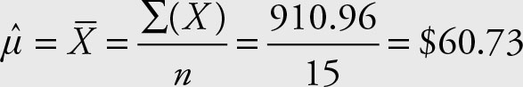
Find the (sample) average price for Wal-Mart for the period from April 2 to April 21, 2012.
Solution
Example 2.3
Suppose the researcher in Example 2.1 collected another sample: The income of these new families is reported below. The researcher wants to calculate the sample mean of their income as well.
65, 57, 71, 72, 63, 71, 65, 55, 71
Solution
The sample mean changed since it is a statistic, which is a variable. This sample mean provides an estimate of the population mean μ. Usually, the parameter remains unknown and statistics provide estimates of it. The mean of combined population can be obtained from the separate component population means. If the researcher considers the 18 observations (of Examples 2.1 and 2.3) as one sample, the sample mean would be:
The same result can be obtained from previous information:
![]()
The mean of the combined samples is:
In this case, the sample sizes are equal, so simple arithmetic average works fine. In the case of different sample sizes, the weighted average is the appropriate tool.
Later, we will cover two other measures of central tendency called median and mode. The knowledge of the median or the mode of two samples or two populations do not render to such calculation. The median or the mode of combined populations or samples cannot be obtained from the component populations or samples.
Trimmed mean is a modification of the mean. The sample data is sorted and a given percentage, say 5%, of the top and the bottom of the data are discarded, and the regular mean is calculated for the remaining data. This trimmed mean will be less susceptible to the extreme values.
Geometric Mean
The geometric mean is calculated using the following formula.
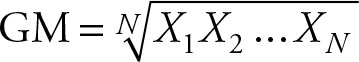 (2.4)
(2.4)
In logarithmic form
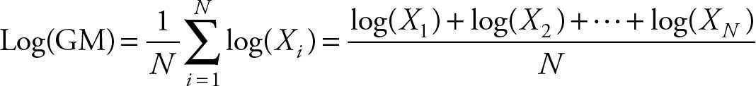 (2.5)
(2.5)
The advantage of the logarithmic formula is that it avoids taking the root of the results. This was more important before the advent of powerful calculators. The logarithmic formula is a linear sum of its elements. After taking the logarithm of the values the mean is calculated as the arithmetic mean.
The geometric mean is useful when the values change in geometric progression instead of arithmetic progression, as is the case with growth rates.
Example 2.4
Assume that a new company grew at 28% the first year, 15% the second year, and 13% the third year. What is the rate of the growth of company?
|
1st year |
1.00 |
beginning of the operation |
|
2nd year |
1.28 |
28% increase over the beginning |
|
3rd year |
1.472 |
15% increase over the 2nd year |
|
4th year |
1.66336 |
13% increase over the 3rd year |
The arithmetic mean is not able to explain the geometric growth. The geometric mean will give the average.
![]()
The company grew at the average rate of 1.4634 or 46.34% per year.
Raise both sides to the 3rd power.
3.134036378 = (1.463416715)3 = (1 + 0.463476715)3
This is the formula for compound interest. To generalize, let P0 be the initial investment, Pn the amount after n years, and r the interest rate or the rate of growth.
Pn = P0 (1 + r)n(2.6)
In the example the ending value is known to be Pn = 3.134036378, the beginning value is P0 = 1.0, and n = 3. The (average) rate of growth is
3.134036378 = 1.0 (1 + r)3

r = 1.463416715 – 1 = 0.463416715
Therefore, the (average) rate of growth is 46.34%, as was derived from the geometric mean.
The geometric mean is also the proper mean when dealing with ratio of items.
Example 2.5
The ratio of the average income to the price of an average car is 4 in year 1 and 5 in year 2. What is the average ratio of income to the price of a car?
Solution
Using the arithmetic mean of income to car price provides an incorrect answer:
(4 + 5)/2 = 4.5
The arithmetic mean of car price to income
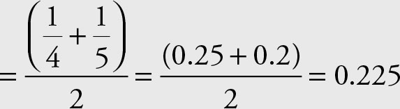
The reciprocal of 0.225 is (1/0.225) = 4.444 not 4.5. Therefore, the arithmetic mean is not a suitable measure when dealing with ratios.
The average of the ratio of income to car price should not differ from the average of the ratio of the car price to income.
The geometric mean for the two ratios is:
Geometric mean of income to car price 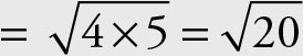
Geometric mean of car price to income 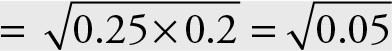
The reciprocal of 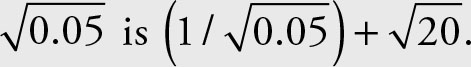 Since the geometric mean of the income to the price of car is the same as the reciprocal of the geometric mean of the price of car to income, the geometric mean is the proper average measure.
Harmonic Mean
The harmonic mean is calculated using the following formula.
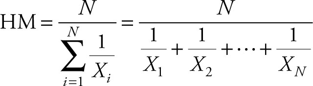 (2.7)
(2.7)
The harmonic mean is, in fact, the reciprocal of the arithmetic mean of the reciprocal of the values.
Example 2.6
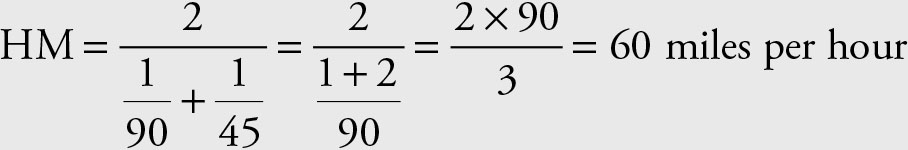
A salesman travels to another city to meet a client. To make sure that he does not miss the appointment, he drives at 90 miles per hour. After a successful meeting he returns more leisurely at 45 miles per hour. What was his average speed?
Solution
The speed was not (90 + 45)/2 = 67.5 mile per hour. For simplicity, assume he traveled a distance of 90 miles (any other value will work as well).
Time while going = 
Time while returning 
Total travel time = 1 + 2 = 3

The harmonic mean will give the correct answer where the arithmetic mean failed.
Rule 2.1
When n = 2 the geometric mean is equal to the square root of the arithmetic mean times the harmonic mean.
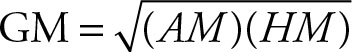 (2.8)
(2.8)
Mean for Data with Frequencies
The expanded presentation below will be revealing.
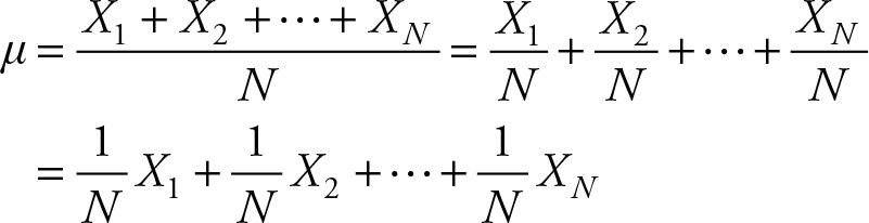 (2.9)
(2.9)
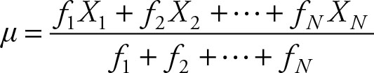
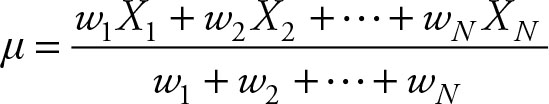
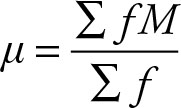
The mean is the sum of 1/N times of each observation. In other words, each observation gets a weight equal to 1/N of the total. Sometimes, each value should receive a different weight, say, f1, f2, …, fN for each of X1, X2, …, XN. In that case the result is in terms of frequencies of each value.
μ = f1X1 + f2X2 + … + fN XN = Σf X(2.10)
Note that Σf = 1 and, hence, was not written. In general, the formula for the frequencies would be:
 (2.11)
Weighted Mean
The weighted mean is similar to the mean using the frequencies, except that the sum of weights need not add up to one.
 (2.12)
Example 2.7
Refer to Example 2.1 and Example 2.3 regarding the incomes of gold miners from two samples.
66, 58, 71, 73, 64, 70, 66, 55, 75
65, 57, 71, 72, 63, 71, 65, 55, 71
List the data according to incomes and their frequencies in a table. Use the number of cases, which is the same as frequencies in this example, as weight and calculate the weighted average.
Solution
This example is exactly the same as Example 2.8, except in the way the number of times an income is named. Here, they are considered as weights for each observation while in Example 2.8 they are considered frequencies.
Recall that the sample mean for the 18 men is

The mean obtained by using the frequency distribution shown in the following table should be the same.
|
Observation |
Weights |
|
55 |
2 |
|
57 |
1 |
|
58 |
1 |
|
63 |
1 |
|
64 |
1 |
|
65 |
2 |
|
66 |
2 |
|
70 |
1 |
|
71 |
4 |
|
72 |
1 |
|
73 |
1 |
|
75 |
1 |
|
Total |
18 |
Adding up the observations and dividing by 12 will give an incorrect answer, except for coincidence. To obtain the correct mean, each observation must be multiplied by the number of times it occurs.
Note that the sum for the population is over the population size N, while the sum for the sample is for the sample size n.

Relation Between Arithmetic, Geometric, and Harmonic Mean
HM ≤ GM ≤ μ(2.13)
The equality sign holds only if all sample values are identical.
Mean of Grouped Data
Statistics is the science of summarizing information. This goal is attained at several stages. The frequency distribution is a tabular summary of data. The mean is another summary statistics that is much more powerful in representing the data. Often, the data are only available after being summarized as frequency distribution. In those cases, it is desirable to be able to find the mean and other valuable parameters.
Mean of Data Summarized as Frequencies
The formula for the population mean is:
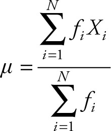 (2.14)
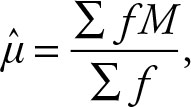
The formula for the sample mean is:
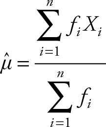 (2.15)
Example 2.8
Refer to Example 2.1 and Example 2.3 regarding the incomes of gold miners from two samples.
66, 58, 71, 73, 64, 70, 66, 55, 75
65, 57, 71, 72, 63, 71, 65, 55, 71
List the data according to incomes and their frequencies in a table. Calculate the mean using the values and their frequencies.
Solution
Using the table from Example 2.7 and multiplying the observations with the frequencies, we have
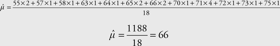
Therefore, summarizing the data into a frequency distribution does not affect the mean. It does not affect the variance either. The mean of the grouped data, however, will most likely be different than the actual mean. This is due partly to the fact that the class sizes are arbitrary, and mostly due to the formula.
Mean for Grouped Data
The formula for the mean of the population grouped data is:
 (2.16)
The formula for the mean of the sample grouped data is:
 (2.17)
where M is the mid-point of each class. Once again the only difference between the population and sample formulas is in the number of elements and where they originate. This is the same as the weighted mean where the weights are the frequencies. Each value is given a weight equal to its number of occurrences or frequency.
Example 2.9
Group the data from Example 2.1 into four groups, each representing a 5-year interval. Calculate the mean using the grouped data.
Solution
|
Classes |
Frequency |
M |
|
55–59 |
4 |
57 |
|
60–64 |
2 |
62 |
|
65–69 |
4 |
67 |
|
70–75 |
8 |
72.5 |
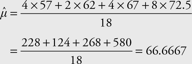
The result has changed slightly. Other groupings will result in different calculated means.
Quartiles
Quartiles divide data into quarters. The first quartile is such a number that 24% of data are below it. Similarly, 50% of data are below the second quartile and 75% are below the third quartile. To obtain quartiles, sort the data and find 1 quarter, 2 quarters, and 3 quarters demarcations. See Examples 2.10 and 2.13 for numerical solutions.
Median
The median is such a value greater than 50% of the population. To obtain the median, sort the data—the one in the middle is the median. If there are two numbers at the middle, their average is the median. Some texts use M to designate the median. The median is the same as the 50th percentile, as well as the second quartile.
Example 2.10
Refer to Example 2.1 and Example 2.3 regarding the incomes of the gold miners in two communities. Calculate the median for each community separately. Find the median for combined data.
66, 58, 71, 73, 64, 70, 66, 55, 75
65, 57, 71, 72, 63, 71, 65, 55, 71
Solution
To obtain the median of each group, sort the values first. The medians for the following two data sets are in bold letters.
55, 58, 64, 66, 66, 70, 71, 73, 75
55, 57, 63, 65, 65, 71, 71, 71, 72
The median of combined population cannot be obtained from the separate component population medians.
55, 55, 57, 58, 63, 64, 65, 65, 66, 66, 70, 71, 71, 71, 71, 72, 73, 75
The median is (66 + 66)/2 = 66.
Mode
The mode is another measure of central tendency. The mode is the most frequently occurring value of the population. A population, or a sample, may have more than one mode or no mode at all. If all members of the population occur as frequently, either no no mode is present or every element is a mode. If there are two modes, the distribution is called bimodal. When the incomes of men and women are measured, there will be two modes, one for men and another for women.
Example 2.11
For data in Example 2.1 and Example 2.3, obtain the mode for the incomes of the two communities. Find the mode for the combined data as well.
Solution
66, 58, 71, 73, 64, 70, 66, 55, 75
65, 57, 71, 72, 63, 71, 65, 55, 71
The mode for the first community is 66, and for the second community is 71. From the frequency distribution table provided in Example 2.7 the mode for the combined data is 71.
The mode of combined population cannot be obtained from the separate component population modes. When the data is grouped, the mode is the midpoint of the interval with the greatest frequency. In a bar graph or a histogram, the tallest bar represents the modal value. In this case the range 70–75 years is the mode.
Empirical Relation Between Mean, Median, and Mode
Mean – Mode = 3 (Mean – Median)(2.18)
Measures of Dispersion
Range
The range is a measure of dispersion. It reflects how far the data are scattered. It is calculated by subtracting the minimum value from the maximum value.
R = Maximum – Minimum(2.19)
Example 2.12
For the data in Example 2.1 and Example 2.3, obtain the range for the combined data.
66, 58, 71, 73, 64, 70, 66, 55, 75
65, 57, 71, 72, 63, 71, 65, 55, 71
Solution
R = 75 – 55 = 20
Interquartile Range
The interquartile range is a measure of dispersion that measures the distance between the first and the third quartiles.
IQR = Q3 – Q1(2.20)
Example 2.13
For the data in Example 2.1 and Example 2.3, obtain the interquartile range for the combined data.
66, 58, 71, 73, 64, 70, 66, 55, 75
65, 57, 71, 72, 63, 71, 65, 55, 71
Solution
Combine and sort the data.
55, 55, 57, 58, 63, 64, 65, 65, 66, 66, 70, 71, 71, 71, 71, 72, 73, 75
Q1 Q2 Q3
IQR = 71 – 63 = 12
The IQR can be used to find the “middle class” of a population or a sample. It gives the lower and upper limits of the middle 50%.
Variance
The variance is a measure of dispersion. It is one of the more important parameters of a population. The concept of variance is used in many aspects of statistics.
The variance is the average error, squared. The need for the variance arises from the need to determine and calculate the error, which is an important statistical measure. The population mean is the best representative of the population. It represents the typical value or the expected value of any member of the population. Seldom, however, every member of the population has the identical value. If they did there would not be any point in studying and analyzing them. Each member of the population will be off from the expected value by some magnitude. The deviation may be positive or negative. Understanding and analyzing the individual errors would be difficult. Instead, the average error is used. As with other subjects in statistics, the goal is to reduce the phenomena to as few parameters as possible.
This section deals with the raw or ungrouped data. The total error and, hence, the average error is always equal to zero. As a mathematical property Σ(X – μ) = 0. To overcome this problem the deviations are squared to obtain:
Σ(X – μ)2
This value cannot be zero unless every observation is identical. Since larger populations will have larger sum of squared deviation, their average is calculated to enable comparison of different sized populations.
Population Variance
The variance is the sum of the squares of the deviations of values from their mean, divided by population size. Therefore, the variance is the mean of the squared deviations, which in the case of a sample it is called the mean squared error (MSE) and, hence, is an average measure. The variance is the entire variation in a population. It does not change.
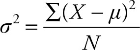 (2.21)
The variance is also called “sigma squared” to reflect the fact that it is a squared measure. The variance reflects (the square of) how much a data point can deviate from the expected value, that is, the mean for the data. The numerator, the sum of squares of deviations, is usually called sum of squared total (SST).
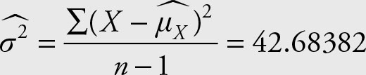
The sample variance is the sum of the squares of the deviations of values from the sample mean divided by the degrees of freedom. The concept of degrees of freedom is discussed in Chapter 3. The sample variance represents the entire variation in a given sample. Sample variance does not change for a given sample. As sample variance is a statistic, its value will change from one sample to the other.
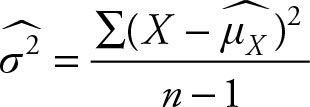 (2.22)
Example 2.14
Refer to the gold miners income data of Example 2.1 and Example 2.3:
66, 58, 71, 73, 64, 70, 66, 55, 75
65, 57, 71, 72, 63, 71, 65, 55, 71
Calculate the sample variances of the incomes for each community.
Solution
The sample variance for the first community is calculated as follows:
|
Income |
|
|
|
66 |
–0.44444 |
0.197531 |
|
58 |
–8.44444 |
71.30864 |
|
71 |
4.555556 |
20.75309 |
|
73 |
6.555556 |
42.97531 |
|
64 |
–2.44444 |
5.975309 |
|
70 |
3.555556 |
12.64198 |
|
66 |
–0.44444 |
0.197531 |
|
55 |
–11.4444 |
130.9753 |
|
75 |
8.555556 |
73.19753 |
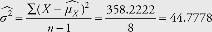
Similarly, the sample variance for the second community is calculated and is equal to
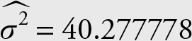
Verify that the variance of the combined samples is neither the sum of the variances of the samples, nor the average of their variances. You can also easily verify that the sum of ![]() equals zero, which will be useful in later discussions.
equals zero, which will be useful in later discussions.
Standard Deviation
The variance, of the population or sample, is in the square of the unit of the measurement of the observation. To make them comparable to the actual observation their square roots is taken.
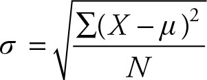 (2.23)
The σ is called the standard deviation. Its counterpart is called sample standard deviation and is denoted by ![]() pronounced sigma hat.
pronounced sigma hat.
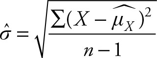 (2.24)
The standard deviation represents the average error of a population or sample. The standard deviation is a measure of risk, too. It reflects how much a data point can deviate from the expected value, that is, the mean of the data, by chance. The standard deviation is the statistical “yardstick” that allows comparison of dissimilar entities. To measure the length of a room, place a yardstick at one end of the room; mark the floor at the end of the yardstick, move the yardstick to the mark, and mark the floor at the end of yardstick again, until the entire length of the room is measured. In other words, you divide the length of the room by the length of the yardstick, and the result will be a value in terms of the yard. The divisor provides the unit of measurement. Hence, the unit of measurement of standardized values is standard deviation.
The Standard Deviation of the Sample Mean
When the value under consideration is the sample mean, its distribution is explained by the sampling distribution of the sample mean, a topic which is covered in detail in Chapter 5. For the time being, we will simply provide the relationship without the background information:
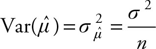 (2.25)
If the population variance is not known, replace it with the sample variance:
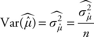 (2.26)
where σ2 is the population variance and ![]() is the sample variance.
is the sample variance.
Definition 2.2
The square root of the variance of the sample mean is called the standard deviation of the sample mean. It is also called the standard error.
Error
In statistics, error is the amount each data point misses the expected value or the average. To avoid using error for two different things, σ, or the standard deviation, is called the error and the (X - μ)2 / N is called the variance or MSE. The term “MSE” is usually used in situations where part of the variation in data can be explained by trend line, treatment, block effect, and so forth, and the remaining unexplained portion is called MSE. The term “variance” is more commonly used for the population variance, when no portion of it could be explained by other factors.
The expected value is the parameter that represents the population. The actual observations deviate from their mean due to random error. The random error cannot be explained. In statistics, it is called the error. The error is the portion of the total variation that cannot be explained. The error is not necessarily a fixed amount. It is the amount not explained by the given tool. Change the tool and the error might change.
Some Algebraic Relations for Variance
Two important relations are used in dealing with variances and are worth reviewing.
1.The variance of a constant is zero.
Var (C) = 0(2.27)
2.The variance of a constant multiple of a variable is equal to the square of the constant times the variance.
Var (CX ) = C2 Var (X )(2.28)
Computational Formula (Short-Cut)
The definitional formula for variance may result in lots of rounding off, especially for a large population or sample, and cause an erroneous difference. If the mean is a never ending real number, the deviation will be a never ending real number. When this deviation is squared and added up, the small amount can add up and give a great bias. The computational formula(e) delay dividing the values as long as possible and do not introduce rounding off into the computation until the last stages.
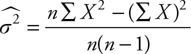
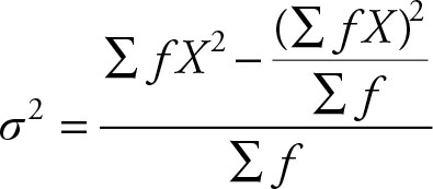
The computational formula for the population variance is
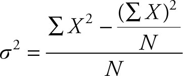 (2.29)
The derivation of the computational formula is relatively simple. It is important to point out that the letters X, N, and so on are dummy notation and are used to represent a variable. Sometimes other letters, such as Y and M, might be used instead. The concept is the same, only the notation is different. Therefore the variance can also be written as:
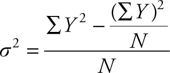 (2.30)
Another computational formula delays division another step.
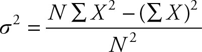 (2.31)
The derivation of this formula is no more difficult than the previous one. The corresponding computational formulas for the sample variance are:
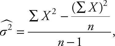 (2.32)
this is the more commonly used formula in most texts
or
 (2.33)
Example 2.15
Use the family income of gold miners from Example 2.1 and Example 2.3 to calculate the sample variance for the incomes of gold miners using the computational formula.
|
Income |
X2 |
|
66 |
4356 |
|
58 |
3364 |
|
71 |
5041 |
|
73 |
5329 |
|
64 |
4096 |
|
70 |
4900 |
|
66 |
4356 |
|
55 |
3025 |
|
75 |
5625 |
|
598 |
40092 |
Solution
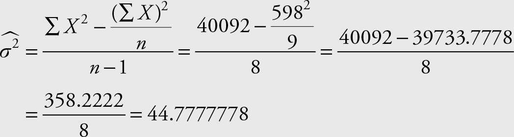
Or
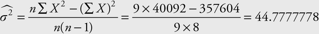
In this example the choice of the formula did not make any difference to the accuracy of the results.
Average of Several Variances
Sometimes it is important to average several variances. Suppose two or more samples are taken from the same population and estimated (sample) variances are obtained. In order to gain a better estimate of the population variance, all the variances should be averaged. If the sample sizes are the same, a simple average will provide the desired mean. If sample sizes are different, however, the observations, which in this case are the variances, should be weighted. The logical weight is the sample size, but since we are dealing with variances and unbiased estimates of population variance come from sample variance, which uses the degrees of freedom as the divisor, the weights to obtain the weighted mean of several sample variances are the degrees of freedom associated with each sample variance. This weighted mean of variances is usually called “pooled” variance. Recall that the formula for weighted mean is:
 (2.34)
Since we are dealing with the variances, and the customary name for the weighted average of variances is called “pooled variance,” and since we use S2 for sample variance we will use the commonly used symbol  The weights (w1, w2, …, wn) are degrees of freedom, and the Xs are sample variances,
  Let n1, n2,… nn be sample sizes. The formula for the case of two sample (estimated) variances is:
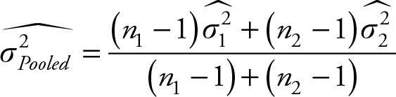 (2.35)
Repeat the pattern to average three or more sample variances.
Example 2.16
Calculate the weighted variance for the variances of the Microsoft stock prices between March 12 and March 30, 2010, and April 2 and April 21, 2012.
Solution
We already have the following results:
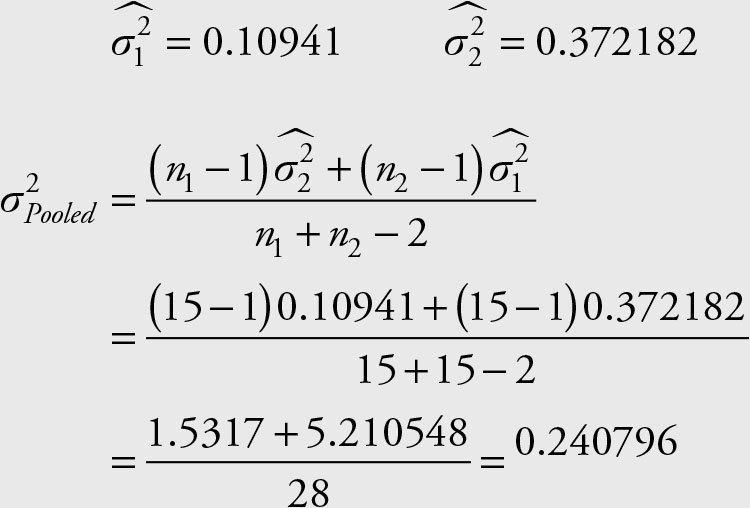
In this and similar examples when the sample sizes are the same the use of weighted average and simple arithmetic average will be the same. Pooled variances are used in the test of hypothesis of equality of two means, as will be seen in Chapter 7.
Variance of Data with Frequency
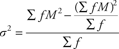
Statistics is the science of summarizing information. This goal is achieved at several stages. The frequency distribution is a tabular summary of data. Often, the data are only available in frequency distribution format. In those cases it is desirable to be able to find the variance and other valuable parameters. The formula for the population variance for the frequency distribution is:
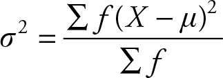 (2.36)
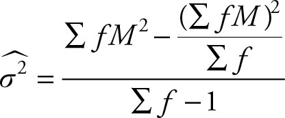
The formula for the sample variance for the frequency distribution is:
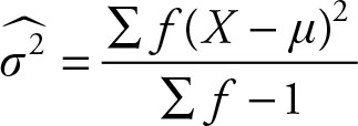 (2.37)
where f represents the frequency of each variable. The limits of Σ for population is N, while that of sample is n.
The computational formula for the population is:
 (2.38)
The computational formula for the sample is:
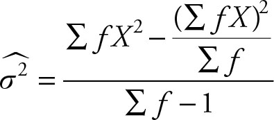 (2.39)
Example 2.17
Use the family income of gold miners from Example 2.1 and Example2.3 that to calculate the sample variance for the first community using the frequency table.
66, 58, 71, 73, 64, 70, 66, 55, 75
65, 57, 71, 72, 63, 71, 65, 55, 71
Solution
Remember from Examples 2.1 and 2.7 the sample variance for these 18 men is equal to
Suppose the raw data is presented in the frequency distribution form.
|
Observation |
Frequency |
|
55 |
2 |
|
57 |
1 |
|
58 |
1 |
|
63 |
1 |
|
64 |
1 |
|
65 |
2 |
|
66 |
2 |
|
70 |
1 |
|
71 |
4 |
|
72 |
1 |
|
73 |
1 |
|
75 |
1 |
|
Total |
18 |
Note that there are 18 observations and not 12. The sample variance for the combined data is equal to 40.23529412. The calculation of the sample variance for the above data using the computational formula follows.
|
X |
f |
xf |
X2 |
X2f |
|
55 |
2 |
110 |
3025 |
6050 |
|
57 |
1 |
57 |
3249 |
3249 |
|
58 |
1 |
58 |
3364 |
3364 |
|
63 |
1 |
63 |
3969 |
3969 |
|
64 |
1 |
64 |
4096 |
4096 |
|
65 |
2 |
130 |
4225 |
8450 |
|
66 |
2 |
132 |
4356 |
8712 |
|
70 |
1 |
70 |
4900 |
4900 |
|
71 |
4 |
284 |
5041 |
20164 |
|
72 |
1 |
72 |
5184 |
5184 |
|
73 |
1 |
73 |
5329 |
5329 |
|
75 |
1 |
75 |
5625 |
5625 |
|
18 |
1188 |
79092 |
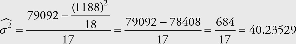
The answer is the same as the one obtained using raw data. Therefore, summarizing the data into frequency distribution does not affect the variance, which will be addressed shortly. It does not affect the mean of the data arranged in a frequency distribution form either. The variance of the grouped data, however, will most likely be different than the actual variance. This is due partly to the fact that the class sizes are arbitrary, and mostly due to the formula.
Variance for Grouped Data
The formula for the variance of the grouped data for the population is:
 (2.40)
where M is the midpoint of each class. The formula for the variance of the grouped data for the sample is:
 (2.41)
where M is the midpoint of each class. The main difference between the two computational formulas is the denominator and the range of summation. The sum for the population covers the members of the population, N. The sum for the sample covers the members of the sample, n.
Measures of Associations
The measures of association determine the association between two variables or the degree of association between two variables.
Covariance
Population Covariance
The covariance is a measure of association between two variables. Let the variables be X and Y and their corresponding means be μX and μY . The covariance is defined as:
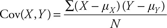 (2.42)
The covariance is the sum of the cross product of the deviations of the values of X and Y from their means divided by the population size. Sometimes it is written as σXY for the population covariance. This is not a standard deviation—it is the notation that reflects that the covariance has a sum of the cross products term. This compares to the notation of ![]() for the variance of the population and σX for the standard deviation of the population.
for the variance of the population and σX for the standard deviation of the population.
The definitional formula for covariance suffers from the roundoff error and also can become very tedious if the means have long decimal places. The computational formula for covariance is:
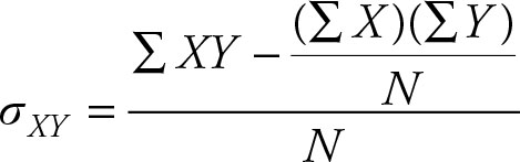 (2.43)
The derivation of the computational formula is not difficult.
Sample Covariance
In the sample covariance the population means are not known and have to be replaced by the sample means. Consequently the covariance loses a degree of freedom. The theoretical formula for the sample mean is:
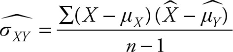 (2.44)
The computational formula for the sample covariance is:
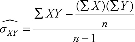 (2.45)
The derivation of Equation 2.45 is identical to the derivation of Equation 2.43. The covariance shows association between two variables. The magnitude of the covariance is a function of the degree of association as well as the units of measurement of the values. The size of covariance will change if the units of measurement are changed, for example from feet to inches or to yards.
Correlation Coefficient
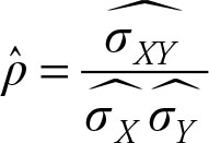
The correlation coefficient ρ uses the measures of association and dispersion to provide a measure without a unit. The measure of association is the covariance and is placed on the numerator. The measures of dispersion are the standard deviation of the X and the standard deviation of the Y, which are placed in the denominator. All three are subject to change when the unit of measurement changes, but the correlation coefficient is immune.
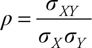 (2.46)
where σXY is the covariance, σX is the standard deviation of the X values, and σY is the standard deviation of the Y values.
The sample correlation coefficient r is written as
 (2.47)
Substituting the formulae for the population covariance and the standard deviations will yield:
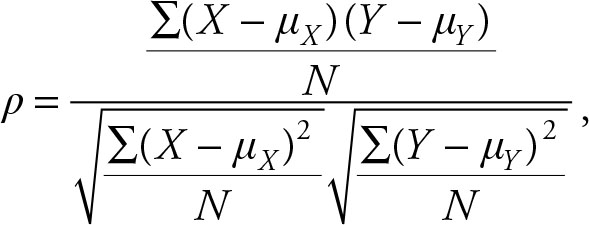 (2.48)
The corresponding formula for the sample correlation coefficient is:
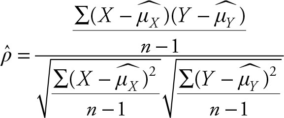 (2.49)
The corresponding computational form for the population and the sample are given in Equations 2.50 and 2.51 respectively.
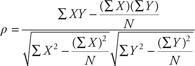 (2.50)
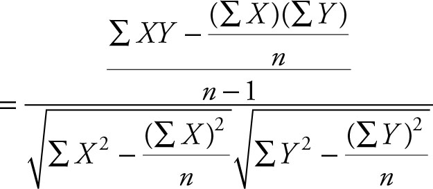 (2.51)
Notice that the only difference between the population and the sample correlation coefficient in the computation formulas is the use of N instead of n. Each is the size of its corresponding data. The difference is conceptual and reflects their origin. Do not overlook the fact that ρ is a parameter and a constant, while r is the statistics and a variable. The sample correlation coefficient r is used to estimate and draw inference about the population correlation coefficient ρ.