
CHAPTER 8
Business Models
Sol comes to the class today with exciting news. A new customer at her Solarists store wants to sign a contract with her company in a joint production process. The customer will start a new company called Photoics that installs the photovoltaic systems for the city residents while her company will provide solar panels. For inventory planning, her boss wanted her to forecast the demand of the photovoltaic systems. Unfortunately, data on the photovoltaic demand for the city are very limited because this is a new product. How can she solve the problem?
Dr. Theo is very glad that she raises the question. He says that one of the sections in this chapter will address her problem. Several business models of the associative analyses using either nonregression or regression techniques will be introduced. Upon completion of the chapter, we will be able to:
1.Analyze the concept of operational forecasting.
2.Describe each of the financial forecast techniques.
3.Explain the two diffusion models to forecast sales and demand for a new product.
4.Apply Excel commands while forecasting the models in (1), (2), and (3).
We are looking forward to learn these practical models.
Operational Forecasting
Operational forecasting involves various departments in a company such as manufacturing, input purchases, marketing, sales, and so on. Krueger (2008) introduced a running forecast technique, of which a simplified version is summarized in this section.
Running Forecasts
Dr. Theo explains, “In a running process, forecasts are calculated for the coming multiple periods but are revised each period throughout the horizon. For example, a company can start from January and calculate forecasts for the next 12 months. The full cycle repeats by the following January. However, the forecasts are revised each month throughout the next 12 months. This is another forecast of forecast technique, where demand for a company’s product has been forecasted using any of the techniques introduced in the previous chapters. Based on the demand forecasts, the company develops operational plans to order inputs, deliver its products, or post advertisements for its coming products.”
Dr. Theo then asks, “Is there any of you who is familiar with the technique?” Arti raises her hand to share her experience. Her Artistown School usually orders books from nationwide suppliers to sell to its students. In the past, they ordered exactly the same number of books every month. Since enrolling in this class, she has been able to forecast the student demand more accurately. She now looks forward to learning this forecast of forecast technique so that she can efficiently place book orders. For the instructional purposes, she shows us a full dataset in the file Ch08.xls, Fig. 8.3.
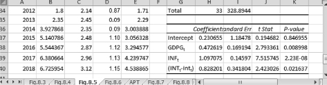
Figure 8.3 Forecasting interest rates: regression results and forecasts
Data Source: Federal Reserve.com (2014).
Dr. Theo picks the first four months of the dataset and makes a simplification by rounding the number of books to the nearest tens. This subset is displayed in Table 8.1 and can be calculated using a handheld calculator.
Table 8.1 Artistown School: balance sheet before book orders are placed
| (1) | (2) | (3) | (4) | (5) | (6) | (7) |
| Month | Forecast | Inventory | Reserve | Balance | Order | Arrive |
| December | 100 | |||||
| January | 30 | 100 − 30 = 70 | 30 * 0.5 = 15 | 70 − 15 = 55 | 0 | 0 |
| February | 40 | 70 − 40 = 30 | 40 * 0.5 = 20 | 30 − 20 = 10 | 0 | 0 |
| March | 50 | 30 − 50 = −20 | 50 * 0.5 = 25 | −20 −25 = −45 | 0 | 0 |
| April | 70 | −20 − 70 = −90 | 70 * 0.5 = 35 | −90 − 35 = −125 | 0 | 0 |
Arti points out that in this figure, column (2) reports her forecasts of book demands from January through April. She also says that she calculated these forecasts in the December of the previous year. In column (3) she begins with 100 books, which were the remaining inventory from December. Each of the other values in column (3) is the projected remaining inventory at the end of each month.
Column (4) represents the reserve of books for emergency when demand from the students suddenly increases. At Artistown School, the reserve is 50 percent of the monthly demand. Column (5) is the balance if no book is ordered and so no book will arrive at the studio. For this reason, the values in columns (6) and (7) are all zeros. Arti wants us to help her fill out these two columns.
We look at columns (3) and (4) of this figure and focus on the values in March to discover that there is a shortage of 20 books to satisfy the forecast demand of 50 and another shortage of 25 books for the reserve in March. Hence, the total shortage is 45 books in column (5) if no shipment arrives in March. This total shortage will rise to 125 books if no shipment arrives in April. Dr. Theo points out that the variables in columns (6) and (7) depend on the values in columns (2) through (5). Arti says her school often plans two months ahead for the number of books to be ordered because it takes six to eight weeks for the books to arrive.
We break into groups to discuss the solutions to the problem. Table 8.2 reports these forecasts of book orders to be placed in January and February. The forecasts can be made for a whole year and can be adjusted each month. Because there will be a shortage of 45 books in March, this amount needs to be ordered in January so that they can arrive by March. These 45 books will be added to the remaining inventory of 30 books from February to make an inventory of 75 books. This new book total satisfies both the demand of 50 books in March and the reserve of 25 books. Hence, the balance in March becomes zero.
Table 8.2 Artistown School: balance sheet after book orders are placed
| (1) | (2) | (3) | (4) | (5) | (6) | (7) |
| Month | Forecast | Inventory | Reserve | Balance | Order | Arrive |
| December | 100 | |||||
| January | 30 | 100 – 30 = 70 | 30 * 0.5 = 15 | 70 – 15 = 55 | 45 | 0 |
| February | 40 | 70 − 40 = 30 | 40 * 0.5 = 20 | 30 – 20 = 10 | 80 | 0 |
| March | 50 | 75 − 50 = 25 | 50 * 0.5 = 25 | 25 – 25 = 0 | 45 | |
| April | 70 | 105 – 70 = 35 | 70 * 0.5 = 35 | 35 − 35 = 0 | 80 |
In February, if the school follows the value on the last row of column (5) in Table 8.1, which is −125, and orders 125 books, then there will a surplus of 45 books, which was already ordered in January. Hence, the school needs to adjust the forecast and reduces its order to 80 books (= 125 − 45), which adds to the 25 books remaining from March to make 105 books by April, just enough to satisfy both the demand of 70 books in April and the reserve of 35 books.
We now see that we can continue to obtain our forecasts in a rolling process and so it is called the running forecast technique.
Excel Application
Arti reminds us that Figure 8.1 displays the full dataset of her Artistown School for 13 months and that the data and commands are available in the file Ch08.xls, Fig. 8.3.

Figure 8.1 Artistown School: running forecasts of book orders
Columns B through F are equivalent to columns (1) through (5) in Table 8.1, of which columns (6) and (7) are not displayed in Figure 8.1 because they all contain zero values. Columns H through L are equivalent to columns (3) through (7) of Table 8.2, of which columns (1) and (2) are already in columns B and C in Figure 8.1. Column M is added to calculate cumulative purchases over time. Initially, only the demand forecasts and the remaining inventory in December are known. We need to perform the following steps:
In cell D3, type = D2 − C3 and press Enter
In cell E3, type = 0.5 * C3 and press Enter
In cell F3, type = D3 − E3 and press Enter
Copy and paste the formula in cells D3, E3, and F3 into cells D4 through F15
Copy and paste-special the values in cells D2 through D4 into cells H2 through H4
In cell H5, type = L5 + H4 − C5 and press Enter
Copy and paste the formula in cell H5 into cells H6 through H15
(Ignore the temporary values, which will be adjusted gradually in a running process)
Copy and paste-special the values in cell E2 through E15 into cells I2 through I15
In cell J3, type = H3 − I3 and press Enter
Copy and paste the formula in cell J3 into cells J4 through J15
(Ignore again the temporary values, which will be adjusted gradually)
In cells K3 and M5, type the number 45
In cell L5, type = K3 then press Enter
Copy and paste the formula in cell L5 into cells L6 through L15
In cell M6, type = M5 + L6
Copy and paste the formula in cell M6 into cells M7 through M15
In cell K4 type = ABS(F6) − M5 then press Enter
Copy and paste the formula in cell K4 into cells K5 through K13
(The last order will be in November for the following January)
The final results in cells J5 through J15 of Figure 8.1 should be all zeros
Financial Forecast
Financial forecasting covers any subject related to financial markets such as expected interest rates, yields to maturity in a bond market, rates of returns by holding a stock, assets and liabilities, prices and exchange rates, and so on. Since the topics are numerous, Dr. Theo says we only discuss the most frequently used models in businesses.
Bond Markets
In this section, we discuss two groups of models: The first is based on expectations theory, which assumes that an investor cares only about the expected yield to maturity (YTM) of a bond; the second group adds uncertainty to the interest rate.
Calculating Expected YTM
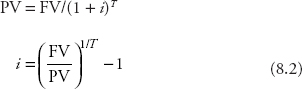
When a company invests in a bond market, the future payment is:
![]()
where FV is the future value, PV is the present value, which is also the price of the bond, i is the interest rate or the expected YTM if the bond is held until it matures, T is the number of years. We can solve for the other variables from Equation 8.1:
The term (1 + i) is called the discount factor, and i is the interest rate, which is the expected YTM in bond markets and which is also called the rate of discount.
At this point, Fin raises his hand to offer an example. A customer came to him to invest $200,000 in a bond market. He offered her a bond that will pay $225,000 in three years. The customer then asks him, “So what is my expected yield per year?” He was able to calculate the YTM for the customer as follows:

The customer was very happy and decided to buy the bond. Fin then says that there are two complicated cases that we cannot calculate the yield so easily. Dr. Theo asks him if he can share his experience with the class. Fin is very happy to oblige, and here is his analysis.
The first case is a fixed payment security, in which a payment on the security is the same every year so that the principal is amortized. The equation for this security is:

where P is the principal of the bond, and F is the future payment.
At this point, Dr. Theo interrupts Fin to remind us that the derivation of Equation 8.3 is in Appendix 8.A. Fin then continues with his discussion.
In this case, you cannot easily solve for i, so the best strategy is to solve for P/F:

Once this ratio is obtained, educational guesses and adjustments have to be made to come up with an expected YTM.
The second case is the coupon bond, which pays a regular interest payment until the maturity date, when the face value (V) is repaid. The equation for this security is:

where P is the price of the bond, F is the future payment, and V is the face value.
In this case, you cannot even solve for P/F and will have to start guessing with the original equation. For Equation 8.4 or Equation 8.5, the guess-and-adjustment process is best worked out on an Excel spreadsheet.
Dr. Theo says that it is very true and that Dr. App will show us the Excel applications later.
Interest Rate Forecasts
Dr. Theo says that in the previous section, we assume that investors only care about their returns. In reality, investors also worry about the risk incurred by a rise in interest rates, which cause the prices of bonds to fall. The uncertainty increases over time, so a term premium is added to the interest rates on long-term bonds.
To account for the risk, we have to forecast the interest rate instead of using a fixed rate. Currently, there are three models for interest rate forecasting (IRF). The first is based on growth theory, which links the interest rate to real GDP growth. The second is based on monetary theory, which links the interest rate to inflation. And the last one is based on financial theory, which links the interest rate to the volatility of the financial market.
Dr. Theo says that we will combine all three into an econometric model using multiple linear regressions. Hence, the equation is written as:
![]()
where
| the long-term interest rate on bond i at time t | |
| GDPGt = | the growth rate of real GDP at time t |
| INFt = | the inflation, measured by the growth rate of CPI at time t |
| INTt = | the average long-term interest rate (5–30-year U.S. Treasuries) |
| intt = | the short-term interest rate (usually on three-month T-bills) |
| (INTt − intt) = | the term premium, which measures the volatility of the market |
We learn that we can estimate Equation 8.6 as discussed in Chapter 6 to obtain point and interval forecasts and that alternative measures of the interest rate determinants are in Orphanides and Williams (2011).
Stock Market
We are very happy to get to this section. We all think that stock markets are fascinating because of their high returns, random behavior, and competitiveness. It turns out that stock markets are not completely random. There are some patterns that help us predict the market values. Dr. Theo says that this section will introduce the capital asset pricing model (CAPM), the arbitrage pricing theory (APT) model, and the dividend discount model (DDM).
Capital Asset Pricing Model
The CAPM formulates the expected return on a particular stock as a dependent variable of the market risk premium, which is the difference between the average return to the stock market as a whole and the interest rate on a risk-free bond. First introduced by Treynor (1962), a simple version of the model can be constructed as an econometric model for a linear regression:
![]()
where
| the expected return on stock i at time t | |
| rt = | the yield (rate of return) on a risk-free bond, often a treasury bond (T-bond) |
| Rt = | average return to the stock market as a whole |
| (Rt − rt) = | the market risk premium, which measures the volatility of the market |
| βi = | the estimated coefficient of the market risk premium |
All assumptions on simple linear regressions hold. There are also five assumptions on the market:
i.The market is competitive.
ii.There are no transaction costs or taxes.
iii.The investors have all information regarding investment choices.
iv. All investors can borrow and lend without changing the interest rate.
Bollerslev, Engle, and Wooldridge (1988) turn this model into a forecast model, of which a simple version is introduced here:
![]()
where ![]() is the forecast value for the following period. Using this model, an expected return of a stock can be forecasted. For example, if your regression result yields bi = 0.3, and at a particular time t you find Rt = 11%, rt = 1%, then you can calculate the forecast value:
is the forecast value for the following period. Using this model, an expected return of a stock can be forecasted. For example, if your regression result yields bi = 0.3, and at a particular time t you find Rt = 11%, rt = 1%, then you can calculate the forecast value:
![]() = 1% + 0.3 * (11% − 1%) = 4%.
= 1% + 0.3 * (11% − 1%) = 4%.
Thus, the expected return of the stock in the next period is 4 percent. The estimated coefficient of bi reveals the direction and volatility of a stock. If bi > 0, the stock moves in the same direction with the market, and if bi < 0, the stock moves in the opposite direction with the market. Additionally, if bi < |1|, the stock is less volatile than the market, and if bi > |1|, the stock is more volatile than the market as a whole.
APT Model
The APT model is an extension of the CAPM and was developed by Ross (1976). This model allows for more than one explanatory variable. For example, the stock price of an agricultural sector might depend on climate changes and the quality of land. This can be written as an econometric model for multiple regressions:
![]()
where X is any factor that affects the expected return of the stock in question in addition to the market risk premium. Based on the forecast version for the CAPM model, the APT model can also be written as:
![]()
where ![]() is again the forecast value for the following period. The regression results then can be used to calculate the expected return of the stock in the following period.
is again the forecast value for the following period. The regression results then can be used to calculate the expected return of the stock in the following period.
Ex raises his hand and offers an example: His company’s stock depends positively on the income (INC) of its trading partners and negatively on the profits (PRO) of its trading competitors. Performing a regression, he finds that ![]() = 0.4 for the INC coefficient and
= 0.4 for the INC coefficient and ![]() = 0.2 for the PRO coefficient. This year, the growth rate of INC is 3 percent and the growth rate of PRO is 2 percent. Using Rt = 11%, rt = 1%, and bi = 0.3, he forecasts the expected return as:
= 0.2 for the PRO coefficient. This year, the growth rate of INC is 3 percent and the growth rate of PRO is 2 percent. Using Rt = 11%, rt = 1%, and bi = 0.3, he forecasts the expected return as:
![]() = 1 + 0.3 * (11% − 1%) + 0.4 * 3% − 0.2 * 2% = 4.8%
= 1 + 0.3 * (11% − 1%) + 0.4 * 3% − 0.2 * 2% = 4.8%
We are very impressed with Ex’s example, which gives us a feel of a real-life situation. Dr. Theo then moves to the next model.
Dividend Discount Model
The DDM utilizes the present value formulas in the section on “Bond Markets” to calculate a company’s expected price based on the investment value theory by Williams (1938). First introduced by Gordon and Shapiro (1956), the model was modified by Gordon (1959) and so was often called the Gordon growth model. The main idea is that a company’s stock price is worth the sum of all of its future dividend payments. The equation for calculating the expected price of a stock is:
![]()
where
| P = | the expected price of a company’s stock |
| DT = | the expected dividend paid by the company at the end of time T |
| T = | the number of time periods |
| i = | the investor’s discount rate |
The investor’s discount rate is subjective. For example, if you want to receive at least 5 percent return from investing in any security, then your discount rate is 5 percent.
If the actual stock price exceeds the expected one, the stock is overvalued. In this case, you might want to move some of your shares in this stock to a different stock. If the actual stock price is below this expected price, the stock is undervalued, and you can predict that the price of this stock will rise. Therefore, it might be profitable to buy some shares of the stock. For this reason, the expected stock price is also called the intrinsic value or fundamental value of a stock.
Assuming that the company’s profits and subsequent dividends are growing at a constant rate over time:
![]()
where
D0 = the initial dividend
G = growth rate of the company’s profits (Π) and dividends (D)
D0 is known at the beginning, and G can be forecasted using any technique introduced in the previous chapters.
At this point, Cita asks, “How can you obtain Equation 8.12 from Equation 8.11?” Dr. Theo says that the derivation is in Appendix 8.B.
Sol then gives an example: As a part of her retirement plan, her company offers her either investing in the company stock or investing in a savings account that pays 0.3 percent per quarter. The initial quarterly dividend paid by her company four quarters ago is $2 per share, her discount rate is 1 percent per quarter, and the average growth rate of her company’s profits over the past four quarters has been 0.5 percent per quarter. We are able to calculate the expected price of her company’s stock as:
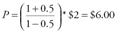
Dr. Theo then tells us to log on to The Wall Street Journal website and look at her company stock price. We find that it is listed on the stock exchange for $2.50 today. Thus, we know that the stock is undervalued, and there is a high probability that its price will rise in the future. Sol is very excited and decides to choose the stock option without delay.
To conclude the section, Dr. Theo reminds us that the assumption of a constant growth rate for both profits and the dividends might not hold in the long run. Thus, the errors might be large, and it is safer to use this model only for short-run forecasts.
Excel Applications
Dr. App reminds us that Figure 8.2 provides a demonstration for bond markets. Columns A through D display calculations for Equation 8.4, and columns F and G display calculations for Equation 8.5.

Figure 8.2 YTM of the fixed payment security and the coupon bond
Expected YTM
Alte offers an example from her Alcorner for the case of fixed payments: A business loan of $25,000 is provided by a local bank to her business. She will repay the bank a fixed amount of $5,000 each year for six years. Dr. App tells us to find out the bank’s YTM at the end of the sixth year. We find the data in the file Ch08.xls, Fig. 8.4, and proceed as follow:

Figure 8.4 Forecasting expected return using CAPM model: regression results
In cell C2, type = A2/B2 and press Enter (hence P/F = 5 as shown in cell C2)
(Try the first calculation with any interest rate, e.g., i = 10% = 0.1)
In cell D2, type = (1 − (1/(1 + 0.1))^6)/0.1 and press Enter
Copy and paste the formula in cell D2 into cells D3 through D9 so that you can try various rates
(The answer, P/F = 4.35526, is too low, so try to reduce i to 0.09)
Double click on cell D3 and change 0.1 to 0.09 and press Enter
Continue to reduce i by 0.01 gradually from cells D4 through D6 where you will see the value 4.91732 which is close to 5
In cell D7, change i from 0.06 to 0.055 and press Enter
In cell D8, change i further to 0.054 and press Enter
In cell D9, change i further to 0.0545 and press Enter
Now you obtain roughly 5.0035, which is at i = 0.0545
Hence, the bank’s YTM is 5.45%
Cita provides an example for the case of a coupon bond: She considers buying a bond that pays $1,200 per year for five years and then repays the face value of $20,000 at the end of the fifth year. The price of the bond is $19,000. She asks us to find the YTM for her.
We try the first calculation again with an arbitrary interest rate i = 10% = 0.1. We find the data in columns F and G of the file Ch08.xls, Fig. 8.4, and proceed as follows:
In cell G2, type = (1200 * (1 − (1/(1 + 0.1))^5)/0.1) + (20000/((1/(1 + 0.1))^5) and press Enter
Copy and paste cell G2 into cells G3 through G9
Continue to reduce i by 0.01 gradually from cells G4 through G9
Cell G9 shows roughly 19,013, and the calculation bar shows i = 0.0721 = 7.21%
Interest Rate Forecasts
Dr. App instructs us to perform a regression of model (8.6) using the data in the file Ch08.xls, Fig. 8.5, and following the commands in the previous chapters. Figure 8.3 displays a section of the regression results and the forecasts for the interest rate on a 10-year U.S. Treasury Bond. We choose the output range of G21 to place the regression results close to cells B36 because the command for the forecasting starts in this cell. From this figure, the estimated equation is:

Figure 8.5 Noncumulative distribution of the product adoption process
![]()
![]()
We find that the forecasts of the explanatory variables are already calculated by Dr. App for our convenience. We only have to perform the following steps to obtain the forecasts:
In cell B36, type = $H$37 + $H$38 * C36 + $H$39 * D36 + $H$40 * E36 then press Enter
Copy and paste this formula into cells B37 through B40
Forecasting Stock Markets
Mo offers us daily data on the prices of his company Motorland stock (MOT). He also shares with us daily data on the market risk premium. The data are for the period from May 1 to May 30, 2014, and are available in the file Ch08.xls, Fig. 8.6. We perform a regression of model (8.8) for the CAPM model and display a section of the regression results in Figure 8.4.
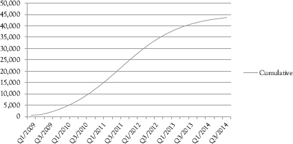
Figure 8.6 Cumulative distribution of the product adoption process
The estimated coefficient of bi is 0.6151, so the estimated equation is:
![]() = −0.1414 + 0.6151 *
= −0.1414 + 0.6151 * ![]()
We then use this equation to calculate the expected returns for May 29 through June 1, 2014: R5/29(MOT) = 0.5607, R5/30(MOT) = 0.5939, and R6/1(MOT) = 0.5380. The values R5/29(MOT) and R5/30(MOT) are for evaluation by comparing them to the actual values.
We see that the results reveal a mean absolute percentage error (MAPE) of roughly 30 percent, which is too large. Dr. App says, “This is the very reason that the model needs to be extended to allow more variables than just the market risk premium.” The regression results also show that the MOT moves in the same direction with the general market (bi > 0), and the former is less volatile than the latter (bi < 1).
We then forecast this stock market using the APT model as shown in (8.10). Since the motorcycle production also depends on aluminum and petroleum prices, these two variables are added to the econometric model with MET as the average daily price of pressed metal companies and PETRO as the average daily price of petroleum companies on the stock exchange. The regression results, which are shown in the file Ch08.xls, on the sheet APT, yield the estimated equation as ![]() =
= ![]() .
.
Substituting the coefficient estimates into this equation, we obtain the forecasts for May 29 through June 1, 2014: R5/29(MOT) = 0.7350, R5/30(MOT) = 0.6915, and R6/1(MOT) = 0.8558. The results reveal a MAPE of roughly 20 percent, which is an improvement compared to the results using the CAPM model. Since stock markets are more volatile than bond markets, this forecast result can be deemed as acceptable.
The estimated coefficients for the two regressions of models (8.8) and (8.10) are quite similar, except that the coefficient for the market risk premium in (8.10) is no longer statistically significant. This implies that the market risk premium might not be the most important determinant of the expected return on the MOT. However, an F-test reveals that the estimated coefficients are jointly significant, so we should not exclude the variable market risk premium from model (8.10) in the regressions and calculations of the forecasts.
Finally, we come to the section that discusses the production adoption process needed for Sol’s forecasts of the photovoltaic demand in the city.
Diffusion Models on Sales and Demand
We learn that the first diffusion model was introduced by Rogers (1962), refined by Bass (1969), and extended by Lawrence and Lawton (1981) to forecast the process of how a new product will be adopted in a population. The models allow a forecaster to generate an entire product life cycle from a few data observations such as the number of the previous buyers and the total market size. Key parameters and their changes can be calculated to obtain the potential demand of a new product prior to the existence of historical sale data.
Sol is very happy that she will not need to collect a long series of the historical data to analyze photovoltaic demand. She shares with us one of the datasets from various cities in the nation to examine the pattern of the product adoption process. We chart the data from the file Ch08.xls, Fig. 8.7, and display the plot in Figure 8.5.
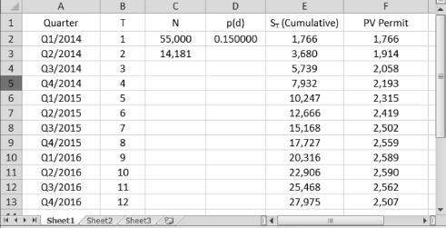
Figure 8.7 Forecasting photovoltaic sales
From this figure, we see that the adoption process has a noncumulative distribution that follows a nearly normal distribution. Dr. Theo tells us that this is the model’s assumption, which might not hold, so the diffusion models usually produce large errors. From this assumption, the cumulative distribution of the adoption is in the form of an S curve. We also chart the cumulative distribution using the data from the file Ch08.xls, Fig. 8.8, and display the plot in Figure 8.6.
From this figure, we see that the cumulative distribution of the adoption process is indeed in the form of an S-curve for this case.
Bass Model
The Bass model is based on the assumption that the timing of a consumer’s initial purchase is related to the number of previous buyers.
Adopters are classified into various categories depending on the timing of their adoptions. The adopters who make the decision to adopt a product early and independently of other adopters are called the innovators. Bass (1969) lists five classes of adopters from the earliest to the latest: (1) innovators, (2) early adopters, (3) early majority, (4) late majority, and (5) laggards. The innovators and the early adopters are the ones who create a diffusion process that results in purchasing by the later adopters. All classes of adopters after innovators are considered imitators.
P(T) is the probability that an initial purchase will be made at time T given that no purchase has yet been made. Then a function with P(T) as the dependent variable can be written as:
![]()
where
| P = | the coefficient of innovation, which depends on factors affecting innovators |
| q = | the coefficient of imitation, which depends on factors affecting imitators |
| m = | the total market potential during the considered period |
| N(T) = | is the number of previous buyers up to time T |
Factors affecting innovators can be advertisements or personal preferences. Factors affecting imitators can be interaction with the innovators or peer pressure. Extended surveys in the past have shown that the average value of p often falls between 0.01 and 0.03, and that the average value of q often falls between 0.3 and 0.5.
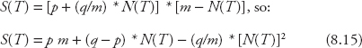
Let f (T) be the likelihood of a purchase at time T, then sales at time T is:
![]()
Combining Equations 8.13 and 8.14 yields:
For example, suppose the total market potential for the iOS8 phones in San Francisco is 120,000 people, the number of previous buyers in the second quarter of 2014 is 10,000 people, quarterly p = 0.02, and quarterly q = 0.4. Then the potential number of sales in the third quarter is:

Lawrence–Lawton Model
Dr. Theo reminds Sol to take notes carefully on this model because it is more refined than the original Rogers and Bass models, so it will help her obtain forecasts of a whole production cycle with only a few observations. Lawrence, Klimberg, and Lawrence (2009) analyze in details five steps of the diffusion process, which is summarized here:
i.Awareness: The potential buyers become aware of the innovation.
ii.Interest: The potential buyers seek additional information.
iii.Evaluation: Enough information is gathered for judgments.
iv.Trial: Samples of the innovation are provided for trying out.
v.Adoption: The adoption process takes place.
The model introduced by Lawrence and Lawton (1981) is for a cumulative unit of sales, S(T), to the end of period T :
![]()
| where N0 = | cumulative number of adopters at time T0 |
| N = | total market potential buyers |
| pd = | a diffusion-rate parameter, which is the speed that the new idea spreads from one consumer to the next |
We break into groups to work on this example: If pd = 0.4, there is a 40 percent possibility that one consumer will tell another consumer in the market about the new product. Suppose the total market for a new brand of camcorders in Korea is 10,000 people, the cumulative number of adopters at the beginning is 1,000 people, the time horizon is two years, and the yearly diffusion rate pd = 0.5, then:

Hence, the cumulative unit of sales for the two-year period is 1,351 camcorders.
In reality, we have to estimate N0 based on the trial sale of the first period S1 = S(1), that is, the number of sales is the same as the cumulative sales in the first period:
![]()
The number of sales in the following periods is:

For example, suppose yearly pd = 0.7, N = 400,000 people; S1 = S(1) = 35,000 for a new brand of computers initially sold in Shanghai, then you can calculate N0 and S(2):
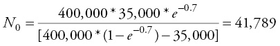

That is, the cumulative number of sales for the two-year period is 89,680 and hence the sale forecast for the second year alone is:
S2 = S(2) − S1 = 89,680 − 35,000 = 54.680 new computers
Excel Application
Since the Bass model can be easily calculated using the mathematical operations for Excel introduced in Chapter 1, Dr. App only provides us with one Excel application for the Lawrence–Lawton model here. Photovoltaic electricity came into existence recently and has developed rapidly in the city. Sol shares with us her data on the photovoltaic permits issued by the city government. Figure 8.7 reveals that the total market potential is N = 55,000 in cell C2.
Since a photovoltaic company does not apply for a permit from the county until a contract with a home owner is signed, this number of permits is a good proxy for the market sales and demand and can be used to forecast future sales and demand.
The sale number in the first quarter of 2014 is the number of permits issued from January 2 to March 30, S1 = S(1) = 1,766, and is displayed in cell E2. Since this is the first period used in the forecast, it is also the first quarterly sale value, which is displayed in cell F2. A survey of the early adopters in the city reveals the quarterly diffusion rate parameter pd = 0.15, which is displayed in cell D2.
We find the data in the file Ch08.xls, Fig. 8.9, and proceed as follows:
In cell C3, type = (C2 * E2 * (EXP(−D2)))/(C2 * (1 − (EXP(−D2))) − E2) and press Enter
(this is the formula to calculate N0)
In cell E3, type = (($C$2 + $C$3)/(1 + ($C$2/$C$3) * EXP(−$D$2 * B3))) − $C$3 and press Enter
(this is the formula to calculate S(2) the cumulative units of sales)
In cell F3, type = E3 − E2 and press Enter
(this is the formula to calculate S2, the forecasted sales for quarter 2)
Copy and paste the formulas in cells E3 and F3 into cells E4 through F13
The forecasts up to the fourth quarter of 2016 are in cells F3 through F13
Dr. App then tells us that monitoring and adjustments are crucial because the actual data provided by Sol are limited to a quarter, so evaluations for long-term forecasts cannot be performed. She confirms Dr. Theo’s remark that the model might produce very large errors if the assumption of nearly normal distribution is violated.
Exercises
1.A CD store in Hong Kong has the forecasts on its CD demand displayed in Table 8.3.
Table 8.3 Forecasts for CD demand
| Week | Forecast | Inventory | Reserve | Balance | Order | Arrive |
| Week 1 | 90 | |||||
| Week 2 | 20 | |||||
| Week 3 | 30 | |||||
| Week 4 | 45 | |||||
| Week 5 | 55 |
Use an Excel spreadsheet or a handheld calculator to fill in the blank spaces and construct another table similar to Figure 8.1 with the reserve values equal 50 percent of the forecast values.
2.A company considers buying a coupon bond that pays $600 per year for six years and then repays the face value of $10,000 at the end of the sixth year. The price of the bond is $9,200. Use an Excel spreadsheet to find out the YTM of this bond.
3.A regression on the return of an automobile company (AUTO) stock on the market risk premium and the changes in oil prices of a petroleum company (PETRO) yields ![]() = 0.75 for the coefficient of the market risk premium and
= 0.75 for the coefficient of the market risk premium and ![]() = −0.2 for the coefficient of PETRO. Additionally, the average return on the stock market as a whole is 9 percent yearly, the average yield on a three-year T-bond is 1 percent yearly, and the growth rate of PETRO price is 4 percent yearly. Use a handheld calculator to forecast the expected return on AUTO stock in the next period.
= −0.2 for the coefficient of PETRO. Additionally, the average return on the stock market as a whole is 9 percent yearly, the average yield on a three-year T-bond is 1 percent yearly, and the growth rate of PETRO price is 4 percent yearly. Use a handheld calculator to forecast the expected return on AUTO stock in the next period.
4.Suppose the total market potential for a new Galaxy tablet in Dubai is 9 million people, the number of previous buyers in the third quarter of 2014 is 1 million people, quarterly p = 0.02, and quarterly q = 0.4 for the Bass model. Use a handheld calculator to forecast the potential number of sales in the fourth quarter of 2014.
5.The Lawrence–Lawton model:
a.A town has the cumulative number of adopters of the iCloud at time T0 = 1300. The market size = 12,000 and the diffusion rate parameter = 0.6. Forecast the yearly cumulative unit of sales up to the end of year 2.
b.Given N = 400,000 people in a city, S1 = 30,000 iClouds, pd = 0.7, use a handheld calculator to calculate N0, forecast cumulative sales S(2), and sale forecast in year 2, S2.
c.Use an Excel spreadsheet to calculate S(1) = St and annual sale forecasts ST for T = 3 through T = 15.
Appendixes
The following appendixes provide the derivations of Equations 8.3 and 8.12 in the section on “Financial Forecast.”
Appendix 8.A Deriving Equation 8.3

where

![]()
Multiplying both sides of Equation A.2 by (1−x) yields:
![]()
Combining Equations A.4 and A.1 yields:
 , which is the expression in Equation 8.3.
Appendix 8.B Deriving Equation 8.12
![]()
Because the growth rate is G,
![]()
Combining Equations B.1 and B.2 yields:
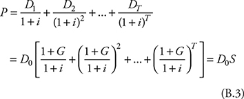
![]()
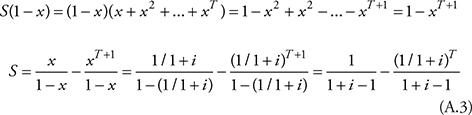
From Equation A.3 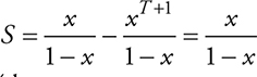 when T approaches infinitive, so Equation B.4 becomes:
![]()
Combining Equations B.3 and B.5 yields:
 , which is the expression in Equation 8.12.