CHAPTER 5

Fiscal Policy

Fiscal policy was introduced with the calculation of fiscal policy multipliers. It is deemed effective in the aggregate expenditure (AE) model of Chapter 3, but not in the aggregate market model of Chapter 4. Although fiscal policy increases aggregate demand (AD) in both frameworks, it raises the price level (PL) in the aggregate market model. The PL is permitted to rise when short-run aggregate supply (SRAS) slopes upward, as it does in Figure 5.1a. When the PL rises, it dampens fiscal policy’s expansionary effect on the real gross domestic product (GDP). This is not the case in the AE model because the PL is held constant when the effects of fiscal policy are analyzed. The constant PL assumption is carried over to the aggregate market model by assuming perfectly elastic SRAS, which is the case in Figure 5.1b.

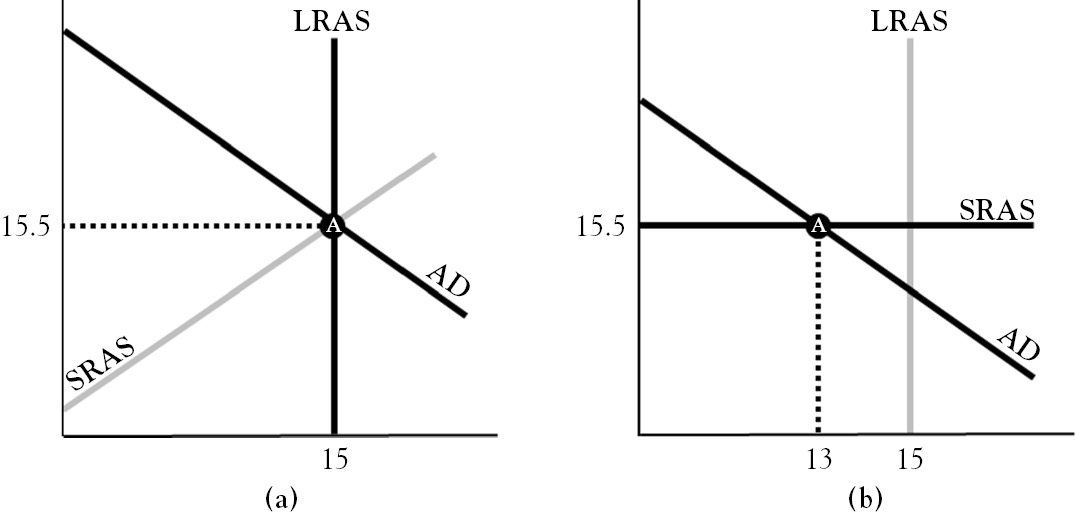
Figure 5.1 Classical economics versus Keynesian economics

The slope of SRAS splits macroeconomics into two major schools of thought. The long-run model of classical economics is shown in Figure 5.1a, while the short-run Keynesian model is shown in Figure 5.1b. In the classical model, SRAS slopes up, intersects AD at long-run aggregate supply (LRAS) due to factor markets clearing in the long run, and is indicated in gray to emphasize the irrelevance of the short run. Keynesian economics assumes that prices and wages are rigid in the short run. This makes SRAS very elastic. It also inhibits resource markets from clearing in the short run, which can make output gaps persistent. Persistently high unemployment in a recessionary gap (point A in Figure 5.1b) and rising prices in an inflationary gap beckon elected officials to alleviate short-run hardships with fiscal stimulus. The attention Keynesians pay to closing short-run output gaps explains why LRAS is gray in the model on the right.

The Fiscal Budget Balance

The fiscal budget balance is the difference between net tax revenue and government expenditure (T − G). The black line in Figure 5.2a is the trend in the real value of the fiscal budget balance by quarter. The budget balance is stated in per capita terms to allow for year-to-year comparisons, which is necessary since the economy and population expand together through time.1 In a given quarter, a budget deficit occurs when the budget balance is negative because government has spent more than it has collected. In such quarters, the trend in the figure tracks below the horizontal axis. A deficit is financed by the U.S. Treasury selling securities, which adds to the national debt. The national debt, roughly 17 trillion dollars in 2013,2 is paid down with budget surpluses. To run a surplus, government cuts expenditure or collects more taxes until the budget balance is positive. This pushes the trend in the figure above the horizontal axis.

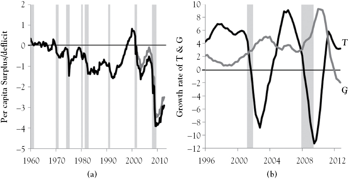
Figure 5.2 Graphs of the fiscal budget balance, growth in T, and growth in G

Prior to the Nixon administration, budget surpluses were common, and budget deficits tended to be small, relative to the size of the population. Eisenhower, Kennedy, and Johnson all presided over surpluses, all of which pale in comparison to Clinton’s. Per capita budget deficits began a fairly consistent downward trend in the Johnson administration. From the late 1960s to just prior to the Great Recession, represented by the right-most gray bar in Figure 5.2, the largest per-capita deficits occurred in Ford’s second full quarter and during the administrations of President Bush and his son. The largest per capita budget deficit in the post-World War II era was recorded near the end of the Great Recession. It was more than twice the size of any other.

With the gray bars in Figure 5.2a indicating recessions, the figure shows the budget balance peaking at the start of recessions and bottoming out at the start of recoveries. Large budget deficits that accompany business cycle troughs shrink rapidly in subsequent economic recoveries and expansions. The figure shows that the celebrated Clinton surplus and its disappearance were driven in part by the business cycle. The surplus peaked in the second quarter of 1999, declined in Clinton’s last two quarters, and continued to fall in his successor’s first quarter, the start of the 2001 recession.3 In the second quarter of 2001, the fiscal budget balance went from being in surplus to being in deficit.

Figure 5.2b disaggregates the fairly recent budget balance story into its two components. The black line in the figure shows the growth rate of per capita tax revenue accelerating until 1997 and then leveling off at around 6 percent per year until 2000. The drop in tax revenue growth to −9 percent began before the 2001 recession started. This drop preceded the enactment of the 2001 Economic Growth and Tax Relief Reconciliation Act (EGTRRA). EGTRRA authorized the Treasury to mail tax rebate checks between July 20 and September 21 of that same year (Snow 2001) and gradually phased in tax-rate reductions between 2002 and 2006 (Dalton and Gangi 2007). The passage of the Jobs and Growth Tax Relief Reconciliation Act (JGTRRA) advanced the 2006 tax rate reductions to 2003. This change was accompanied by tax revenue growing at around 9 percent by 2005. With the lower tax rates set to expire in 2010, the Obama administration extended them to 2012. According to the figure, tax collections are highly correlated with the business cycle.

The gray trend in Figure 5.2b shows the volatility in per-capita government expenditure, which is much smaller than that of tax revenue. After six consecutive quarters of government expenditure growing at a slow rate, its growth rate increased substantially between 1999 and the start of the 2001 recession. The acceleration in earmarks4 (Utt 1999) and the business cycle were large drivers of this. Twenty-six days after the 9/11 attacks, the war on terror was launched. With its cost estimated at over 1 trillion dollars (Belasco 2011), the gray line in Figure 5.2a subtracts out the average annual war appropriation from the budget balance. The government expenditure growth accelerated from 2.4 percent at the start of the 2001 recession to peaks of 5 percent in the second and final quarters of 2003. The enactment of the 3.1-trillion-dollar 2009 budget, the Troubled Asset Relief Program (TARP), the omnibus and other appropriations bills, and tax rebates in the final year of the Bush administration coincided with government expenditure growth jumping to 4 percent. This was followed by an even larger acceleration in government expenditure after the Obama administration enacted the American Recovery and Reinvestment Act and the Omnibus Appropriations Act months apart during its first year.

Figure 5.2 indicates that budget deficits have become the norm in the United States. In the classical view, discretionary changes to the fiscal budget are unnecessary because output gaps are not present in the long run. The Keynesian view, on the other hand, prescribes budget deficits for recessionary gaps, which are to be paid off with budget surpluses during subsequent economic expansions. Given how rare surpluses are, fiscal policy is not being implemented as prescribed by the Keynesian school of economics. This is perhaps a result of cuts in expenditures on government programs being viewed as political suicide by progressive politicians, and hikes in tax rates being viewed as political suicide by conservative politicians.

Treasury Bond Auctions

The U.S. Treasury borrows to cover budget deficits by selling securities to banks, other nations’ central banks and governments, large corporations, and others. U.S. securities include bills, notes, and bonds. Bills mature in 1 year or less, notes in 2 to 10 years, and bonds in more than 10 years. Although U.S. securities are auctioned and redeemed by the U.S. Treasury in what is called the primary market, holders can sell them before they mature in the secondary market. The yield on a U.S. security—the rate of return that accounts for purchase price, coupon payments, and face value (FV)—is considered the benchmark for fixed-income securities with the same attributes because it is considered risk free. The yield curve, the relationship between the yields and maturities of U.S. securities, normally slopes up but flattens as the likelihood of recession rises.

U.S. securities are sold in periodic auctions. In 2012, 264 public auctions worth 8 trillion dollars were conducted.5 This amount is about eight times larger than that year’s budget deficit because the auctions must be large enough to cover the deficit, pay interest payments, and retire maturing securities. After auctions are announced, investors submit bids to the U.S. Treasury. When an auction ends, bids exceeding the winning price are accepted. To demonstrate this, consider a one-year Treasury bill auction intended to raise 1 billion dollars. Suppose the bill has a FV of $100, a maturity (n) of one year, and a price of the winning bid (P) equal to $98.91. Substituting these values into the equation below gives a yield of 0.011 or 1.1 percent.

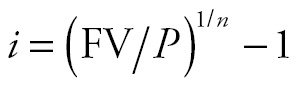
Since the bill sold for $98.91 and the auction intended to raise 1 billion dollars, 10.11 million bills must be issued. If the price of the winning bid had been $99.11, the yield would have been 0.9 percent. Thus, Treasury bills are typically discounted, and their prices and yields are inversely related. Prices and yields of securities with longer maturities are also inversely related, but may not sell at a discount because bearers receive interest (coupon) payments twice a year.

Discretionary Fiscal Policy

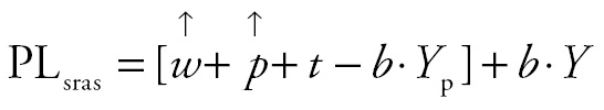
A deliberate change in the budget balance is called discretionary fiscal policy. Figure 5.3 shows its effects on the major macroeconomic models. In classical economics, AD and SRAS intersect at LRAS, point A in Figure 5.3a, because labor and other resource markets clear in the long run. If tax rates are reduced or government expenditure is increased, the budget goes from being balanced to being in deficit. The arrows above G and T in the equation below show how expansionary fiscal policy affects AD.

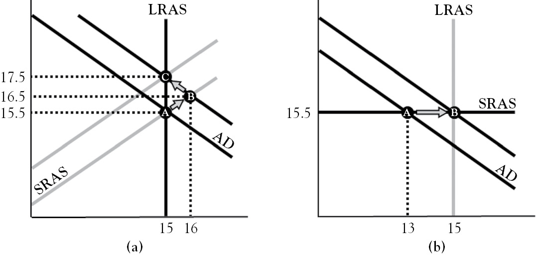
Figure 5.3 Expansionary fiscal policy in the classical and Keynesian schools

Raising the budget deficit increases AD’s intercept, which shifts AD to point B in Figure 5.3a. At this point, the economy is an induced inflationary gap because real GDP exceeds its potential.

At point B, labor markets are tight because unemployment is below its natural rate. If the Fed does not offset fiscal stimulus with tighter money, firms bid wages up. The prices of other production inputs are bid up too due to the heavy utilization of facilities and overemployment of resources. The arrows above w and p in the following equation show how the model self-adjusts.

Rising wages and prices of other inputs to production increase the value of SRAS’s intercept, shifting SRAS from point B to C. At point C, wages and prices of other inputs to production no longer change because resource markets have equilibrated. With real GDP equal to its potential, the PL settles at 17.5 thousand dollars. Thus, in classical economics, expansionary fiscal policy is inflationary, has no effect on real GDP, and increases the budget deficit, which adds to the national debt.

In Keynesian economics, perfectly elastic SRAS and AD intersect at points that are to the left or right of LRAS. SRAS is perfectly elastic because Keynesian economics assumes that wages and prices are rigid in the short run. This makes w and p fixed parameters. In Figure 5.3b, the aggregate market is in a recessionary gap at point A. As in the classical model, an increase in government expenditure or a cut in taxes increases the size of the budget deficit and AD’s intercept. The figure shows that the budget deficit is just enough to close the 2-trillion-dollar recessionary gap. Thus, expansionary fiscal policy returns the economy to full employment, is not inflationary, but raises the national debt by the amount of the budget deficit.

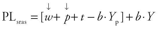
The effects of discretionary restrictive fiscal policy are shown in Figure 5.4. In the long-run classical model on the left, the economy is initially at point A. If taxes are raised or government expenditure is cut, the fiscal budget goes from being balanced to being in surplus. The arrows above G and T in the equation below illustrate how restrictive fiscal policy affects AD.

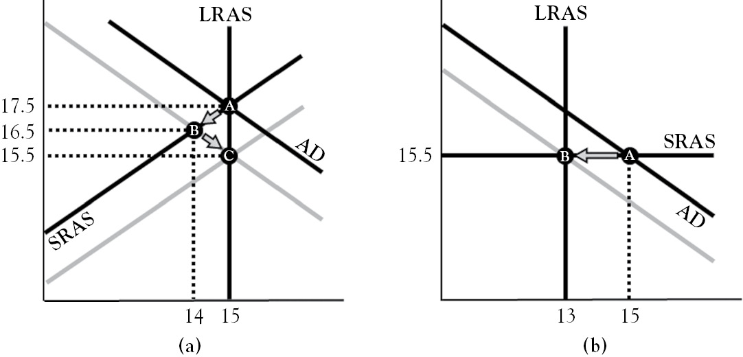
Figure 5.4 Restrictive fiscal policy in the classical and Keynesian schools

Cutting government expenditure or raising taxes reduces AD’s intercept, which shifts AD from point A to B. At point B the economy is in an induced recessionary gap because potential output exceeds real GDP. This causes unemployment to rise above its natural rate, which means that facilities are underutilized and resources are underemployed. Wages and the prices of other inputs fall because government does not intervene in markets in the classical model. The arrows above w and p in the following equation show how the model self-adjusts.

As wages and prices of production inputs fall, SRAS self-adjusts to point C. As real GDP returns to its potential level, the PL drops to 15.5 thousand dollars. Thus, in classical economics, restrictive fiscal policy has no effect on real GDP and is deflationary.

The Keynesian model in Figure 5.4b is in an inflationary gap at point A. As in the classical model, raising taxes or cutting government expenditure decreases AD’s intercept, which shifts AD from point A to B. This implies that restrictive fiscal policy in Keynesian economics can return the economy to full employment and is not deflationary. In addition, the resulting fiscal surplus can then be used to pay off budget deficits that were used to close recessionary gaps.

Shortcomings of Fiscal Policy

Although discretionary fiscal policy is seemingly effective in the Keynesian model, in practice, it is futile. Because forecasting is difficult and gets increasingly unreliable the further into the future predictions are made, fiscal policy will overshoot or undershoot an output gap. If the fiscal stimulus is too small in Figure 5.3b, AD will shift along SRAS to a point between A and B. This leaves the economy in a smaller recessionary gap. If the initial stimulus was too large with the economy at point A, AD will shift along SRAS to a point to the right of point B. This induces an inflationary gap, and requires a withdrawal of stimulus or tighter money from the Fed to prevent SRAS from eventually self-adjusting upward due to resources being overemployed.

Even if the size of discretionary fiscal stimulus is predictable, there are delays in its implementation. It takes time to observe that the economy is in a recessionary gap because GDP and unemployment are not observed in the present. In addition, several months of observations are needed to make an accurate prognosis. After a problem has been diagnosed, it takes time to decide the best course of action because Congress must debate, compromise, amend, and vote on the action to be taken. When the President’s party does not control both chambers of Congress, adopting fiscal policy is very challenging. Even if the President’s party controls the House and Senate, the Senate minority can stop legislation if it gets at least 41 senators to support a filibuster. After fiscal policy is signed into law by the President, its effects are further delayed by revenue from new taxes being collected a year or more after the change was made or by bureaucratic red tape that includes departments altering budgets, adjusting spending habits, and screening grant or transfer payment applicants. Sometimes, its implementation is purposely lagged by several years, with EGTRRA being a great example. Even the theory behind multipliers implies that the economic benefits of fiscal stimulus take time to unwind.

Figure 5.5 shows how poorly timed discretionary fiscal policy can destabilize the economy. SRAS slopes upward because stagflation6 in the 1970s implies that wages and prices are not rigid. At point A, unemployment is equal to its natural rate because real GDP is equal to its potential. Suppose that investment slumps. This is modeled by the arrow above I in the following equation.

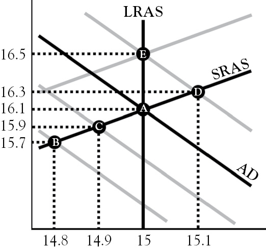
Figure 5.5 Expansionary fiscal policy in the presence of policy lags

If the decline in the intercept causes AD to shift from point A to B, the real GDP falls to 14.8 trillion dollars. As unemployment rises, voters implore elected officials to take action. Complying with this is difficult because certain politicians support a temporary boost in government expenditure while others back tax cuts. As Congress debates a plan of action, suppose that good news from overseas sparks a stock market rally that increases consumer wealth (W ) just enough to push AD to point C. The arrow above W in the following equation illustrates this effect.

With the economy at point C, suppose that the House and Senate start reconciling their stimulus bills. As this continues, the increase in consumer wealth boosts expected future income (Ye) enough to push AD to point A. The arrow in the equation below shows how AD is affected by this.

The increases in consumer wealth and expected future income are enough to return the economy to full employment. Although this typically happens before fiscal stimulus is injected into the economy, repealing the stimulus bill is not politically popular. After the President signs the bill, consumers receive tax cuts and firms get paid for filling orders for new public works projects, and AD shifts from point A to D. If the Fed fails to offset this with tighter money (to push AD back toward point A), overemployment of labor and high resource and facility utilization causes firms to bid up wages and prices of other inputs. These shift SRAS up to point E. Thus, poorly timed fiscal policy adds to the national debt, is inflationary, and, in the end, does not affect real GDP or unemployment.

Discretionary fiscal policy has domestic and international consequences, too. Suppose that a tax cut and increase in government expenditure are able to close the recessionary gap shown in Figure 5.6a. Since these actions increase the budget deficit, government must borrow funds in the loanable funds market depicted in Figure 5.6b. Savers supply loanable funds when they purchase bonds from governments and firms. The price of loanable funds is nominal interest rate i, which is used to compute interest paid to savers. If it is 0 percent, demanders will want to borrow a lot of these funds, but savers will not supply them. As the nominal interest rate rises, the shortage in funds declines as borrowers demand fewer funds and savers supply more. The shortage disappears when the nominal interest rate reaches its equilibrium of 2.5 percent at point A. At the moment government borrows to finance the budget deficit the demand for loanable funds (DLF) shifts to point B. With loanable funds supply (SLF) held constant, higher loanable funds demand pushes the nominal interest rate up to 3.5 percent.

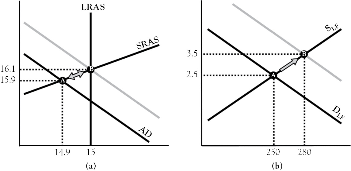
Figure 5.6 Fiscal policy and the crowding-out effect

Foreign and domestic capital is attracted to U.S. securities when real interest rate r is pushed up by a higher nominal interest rate.7 With domestic capital flowing to government securities, less is being invested in new plants, equipment, and homes (I ). Foreign capital flowing into the United States reduces the amount of capital that is invested in other countries. The decline in private investment, here and abroad, caused by an increase in U.S. government borrowing is called crowding out. Since U.S. securities are purchased in dollars, foreign investors swap their currencies for dollars, which causes the dollar to appreciate. This makes U.S. products more expensive abroad, which reduces U.S. exports (X ). The arrows in the following equation show how the consequences of increased government borrowing affect AD.

Although increasing the size of the budget deficit (higher G and lower T ) shifts AD from point A to B in Figure 5.6a, crowding out (higher r and lower X and I) shifts AD back to point A. Hence, the intended consequence of fiscal policy is accompanied by unintended domestic consequences, which consist of higher interest rates and lower investment expenditure, and an unintended international consequence, the decline in exports that is caused by an appreciating dollar.

Although Keynesian economics advocates for countercyclical changes in the budget balance to smooth the business cycle, the continual adjustment of tax rates and expenditures makes it difficult for individuals and firms to plan for the future. Not knowing what tax rates will be next year, in two years, or in five years makes computing expected returns difficult. This retards economic activity and job creation (Meltzer 2012) and hinders long-run economic growth.

Oddly enough, politicians need not take action when the economy slips into recession because there are automatic fiscal stabilizers at work in the economy. Automatic stabilizers are countercyclical effects that are not hindered by legislative delays. Examples of these include progressive income taxation, unemployment insurance (UI), and Supplemental Nutritional Assistance Program (SNAP). As growth accelerates, incomes rise. This means that more and more people are paying an increasing proportion of income in taxes because they find themselves in higher and higher income tax brackets. This dampens consumption expenditure, and limits the peak of the business cycle. As the economy approaches the trough in the business cycle, more and more people are paying less in income taxes—because they find themselves in lower and lower income tax brackets—or are receiving transfer payments from UI or SNAP. As the deficit automatically widens without legislative delay, immediate stimulus is injected into the economy, which pushes real GDP back toward its potential level. The additional tax revenue accruing to the Treasury during an expansion automatically pays down the fiscal deficit resulting from an economic contraction.

The Supply-Side School

At the end of World War II, the views of John Maynard Keynes and F.A. Hayek split economics into two camps. Unlike Keynes, Hayek argued for limited government, economic freedom, and personal responsibility. While Keynes’s view dominated mainstream economic thought and policy formation in the decades following the war, Hayek’s views helped revive classical economics. As this was going on, shifting inflation expectations of the 1970s ushered in stagflation. This revealed that prices and wages were not as rigid as Keynesian theory had assumed. As a result, the aggregate market model became the standard in macroeconomic principles textbooks.

In The Way the World Works, after attributing high tax rates and poor monetary policy to the stagflation of the 1970s, Jude Wanniski made the case for supply-side economics. The theory emphasizes permanent reductions in tax rates and regulations, which fuel continual increases in production capabilities over time. This pushes LRAS and SRAS outward at a pace higher than what would have prevailed under a regime of continuous fiscal policy adjustment. Because the three curves of the aggregate market model equilibrate in the long run, AD shifts outward to keep up with LRAS and SRAS,8 which is shown in Figure 5.7. The figure implies supply-side economic policy results in zero inflation and ever-expanding GDP.

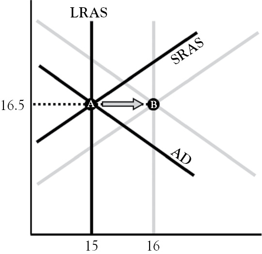
Figure 5.7 Supply-side fiscal policy

The marginal tax rate is crucial in supply-side economics. If the tax rate is 100 percent, people will not work and firms will not produce, resulting in zero taxes being collected. Conversely, people and firms pay zero income taxes when the tax rate is 0 percent. Thus, tax revenue rises and then falls as the tax rate is raised from 0 to 100 percent. This relationship is called the Laffer curve.9 It was the topic being discussed by Ferris’s economics teacher, played by Ben Stein in 1986’s Ferris Bueller’s Day Off, during his infamous day off from high school. The empirical Laffer curves graphed in Figure 5.8 show how tax revenue and the top marginal tax rate relate over time in the United States.10 According to the left figure, tax revenue as a percentage of GDP is maximized when the tax rate is 50 percent. The figure on the right, however, implies that per capita tax revenue reaches a maximum when the tax rate is less than 25 percent. Although both curves suggest that cutting “high” tax rates raises tax revenue, the left curve implies that this only works up to a point. Since real GDP is more volatile than population estimates, and it is highly correlated with tax revenue (see Figure 5.9b), the empirical Laffer curve on the right fits its scatterplot better than the curve on the left.

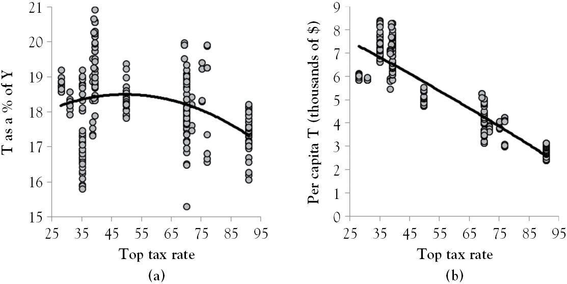
Figure 5.8 Empirical laffer curves

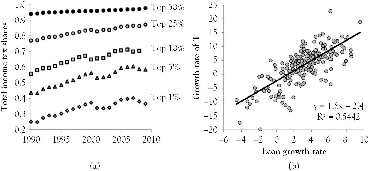
Figure 5.9 Tax burden, and growth in T versus GDP growth

Figure 5.9a11 seems to confirm the Laffer effect. Although it shows that the tax burden borne by those in the top three income brackets is sensitive to the business cycle, the income tax burden borne by those in the top five income brackets generally rises over time. From 2003, the year the EGTRRA income tax rate cuts were completely phased in, to the year preceding the start of the Great Recession, the burden of taxation borne by those in the top two income tax brackets increased rapidly by 5 to 7 percentage points.

The Laffer curve implies that there is a limit to the amount of taxes that can be collected from taxpayers in the short run. Thus, government cannot provide services costing more than this limit unless it runs a budget deficit. Elected officials interested in balancing the fiscal budget and providing services exceeding the limit imposed by the Laffer curve can do so if they enact policies that will shift the curve up. Permanent reductions in tax rates and regulations expand the long-run productive capacity of the economy. This in turn shifts the economy’s PPF outward, rotates the short-run production function counterclockwise, and shifts LRAS to the right. If these policy prescriptions achieve a sustainable economic growth rate of 5 percent, annual tax revenue will grow at the rate of about 7 percent, according to Figure 5.9b.

Since Congress cannot bind future Congresses to the policies it enacts,12 a cut in the payroll tax rate firms pay, a reduction in regulations, or a tax holiday on overseas corporate profits represent discretionary fiscal policy. Thus, any critical evaluation of what are classified as supply-side economic policies is really an indictment of discretionary fiscal policy.

The Chicago School

Hayek’s views also helped shape the Chicago school. It is associated with the following tenets: markets allocate resources more efficiently than do governments, monopolies are created by government regulation, and central banks should maintain low and steady rates of money growth. The Chicago school views fiscal policy as ineffective because households form rational expectations.13 If households do not expect their taxes will be raised to retire the bonds used to finance today’s budget deficit, fiscal stimulus shifts AD toward point B in Figure 5.10a.

Recent experience, however, suggests that households form rational expectations.14 If so, households expect that tax rates will be raised in the future to pay off today’s budget deficit. This reduces expected future consumer income (Ye ). In addition, when government borrows more to cover a budget deficit, demand for loanable funds shifts from A to B in Figure 5.10b. Since households save tax rebates and paychecks earned from public works projects to pay higher future taxes, loanable funds supply shifts from B to C. This keeps the nominal interest rate at 2.5 percent. If the expected inflation is steady, real interest rates and investment expenditure are constant. The arrows in the following equation show how rational expectations offset fiscal stimulus.

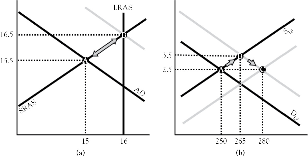
Figure 5.10 Fiscal policy in the presence of rational expectations

Although fiscal stimulus shifts AD to point B in Figure 5.10a, this is completely offset by a decline in expected future income that pushes AD back to point A. Thus, in the Chicago school, fiscal policy has no effect on interest rates, real GDP, or unemployment.

The Austrian School

The 1871 publication of Carl Menger’s Principles of Economics established the Austrian school of economics. Unlike its cousins—supply-side economics and the Chicago school, which advocate a limited role for government in managing the economy—Austrian economics adheres to classical liberalism. To Austrian economists, mainstream macroeconomics is an oxymoron because, to them, the appropriate unit of analysis is at the individual level. This, however, does not preclude Austrians from commenting on macroeconomic issues.

Austrians view the injection of fiscal stimulus into the economy as treating the symptoms of economic malaise rather than being its cure. The Austrian prescription for persistently high unemployment would be painful to low-skilled workers in the short run because it involves the elimination of the policies that make wages and prices rigid.15 The rigidities are a result of government interventions that raise low-skilled laborers’ reservation wages, which include UI compensation (Layard, Nickell and Jackman 1991), the minimum wage and pro-labor policy (Barro 1988), public assistance (Borjas 2012), and price controls present in farm bills (Bakst and Katz 2013). Artificially low mortgage rates and easy credit terms in the early to mid-2000s trapped low-skilled workers in homes in the mid-2000s, which can inhibit migration to low-unemployment regions.

After regulations, subsidies, and other government interventions are repealed, the Austrian solution to recessionary and inflationary gaps is laissez faire policy. It would allow markets to adjust to various dynamics. The resulting changes to prices and wages send clear signals to self-interested individuals. Consider the inflationary gap at point A in Figure 5.11. It and allowing SRAS to self-adjust to point B are viewed as being very beneficial to the economy. This is because firms cannot pass higher labor and resource costs off onto consumers when faced with stiff competition at home and abroad. In the absence of intervention, allowing overemployment to persist drives cost-saving innovation because firms employ individuals who find creative ways to lower production costs. Greater entrepreneurialism and technological advancement shifts LRAS and SRAS to point A. As this occurs, unemployment adjusts upward toward its natural rate as workers are replaced by the adoption of labor-saving technologies.

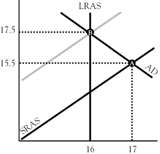
Figure 5.11 Inflationary gaps in the austrian school

Although economic prosperity is linked to core tenets of Austrian economics, namely economic and political freedom, this school of thought is routinely dismissed or marginalized by mainstream economists (e.g., Krugman 2013). This is the case despite prices falling, quality rising, and consumer choice increasing in the long-run in markets that are relatively free of government intervention (e.g., cellular phones, tablets, Internet, electronics, software, and computers). On the other hand, inflation, stagnant quality, inefficiency, or moral hazard is typical of industries regulated, managed, or owned by government (e.g., landline telephones prior to the breakup of Ma Bell, banking, education, healthcare, and the post office). Thus, it is surprising that the Austrian view has not gained wider acceptance. This is perhaps due to mainstream economics offering sellable solutions to recession. While Austrian economics leaves people to their own devices when unemployment is high, mainstream economics does not. Keynesian solutions, like public works projects, extensions to UI compensation, and payroll tax cuts, are well received among working-class voters. Supply-side and Chicago school policy prescriptions, such as capital gains tax rate cuts, low interest rates, and deregulation, appeal to investors and entrepreneurs.

Fiscal Policy and Economic Performance

Due to policy lag, past values of annual budget deficits should impact current economic growth. However, correlations between economic growth rates and quarterly lags of the growth rate of budget balances are essentially zero. A similar story plays out when correlations of economic growth rates and lags of the per capita budget balance are computed. The strongest correlation occurs when the per capita budget balance is lagged by eight quarters. This relationship is shown in Figure 5.11 for the 1986 to 2005 period. The trend line in the figure implies that raising the budget deficit by $2,000 per citizen leads to a modest 0.35-percentage-point increase in economic growth two years later. Given the weak correlation between growth and lags of these budget measures, and the budget balance’s modest effect in Figure 5.11a, other policies should perhaps be pursued.

The persistence of budget deficits in Figure 5.12 suggests that they are politically popular. Near the peak of the Clinton surplus, Congress accelerated its expenditures. Although government expenditures had been growing steadily at 1 percent per year, its growth rate steadily increased to 5 percent between 1999 and 2003. The growth in government spending remained near this elevated rate through 2004 even though the recession had ended three years earlier. Meanwhile, the temporary EGTRRA tax rates had been fully phased in by 2003. In 2008 and 2009, the Bush and Obama administrations enacted stimulus bills and bailed out corporations and banks using TARP funds to rescue the United States’ “financial system from almost certain meltdown [and help] avoid the feared second Great Depression” (Weller 2012). Given that the fiscal stimulus used to combat the 2001 recession was injected late, and the record fiscal stimulus of 2008 and 2009 did not pull the economy out of the deepest and most persistent recessionary gap since the Great Depression (see Figure 2.7), will politicians abandon fiscal policy? Perhaps not, because (a) higher government spending and lower taxes directly benefit their constituents, and (b) they will be long retired by the time the bonds that financed their policies mature.

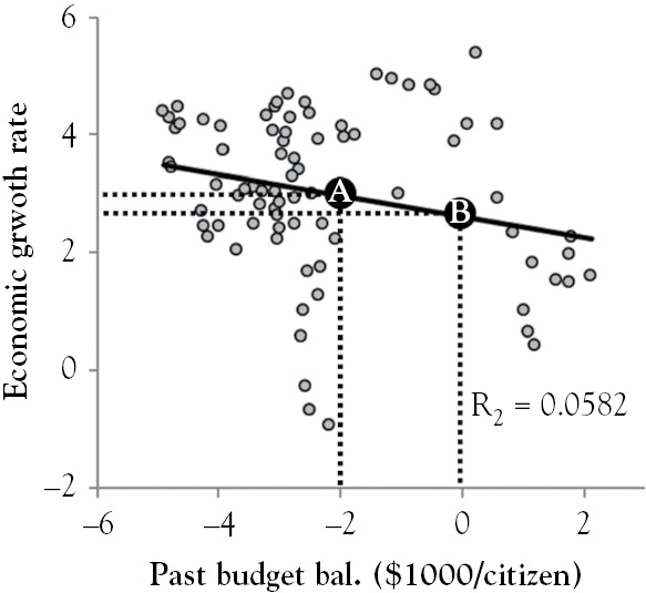
Figure 5.12 Economic growth versus lagged fiscal budget balance