
Aggregate expenditure (AE), summarized in the final column of Table 2.4, is the sum of consumer expenditure, investment expenditure (new home sales and firm investments in new buildings, equipment, tools, and inventory), government purchases of goods and services, and net exports. This definition implies that a recession triggered by a cutback in consumer or firm expenditure can be offset one-for-one with a boost in government expenditure. This notion is the core of Keynesian economics, and assumes that the last dollar government spent building the “Bridge to Nowhere”1 is as productive as the last dollar spent improving computer processors, motion picture sound and visual effects, or the aerodynamics of passenger jets. In his 1974 Nobel Prize acceptance speech, F.A. Hayek said that this kind of thinking has “made a mess of things … [because] it leads to the belief that we can permanently assure full employment by maintaining total money expenditure at an appropriate level.” Despite this and other criticisms, Keynesian economics remains relevant because government expenditure and total employment are strongly correlated;2 it justifies politicians cutting taxes and “spending public monies on projects that yield some demonstrable benefits to their constituents” (Buchanan and Wagner 1999); and its simple elegance makes it easy to teach and understand.
Consumer Expenditure
The consumption function is at the heart of Keynesian economics. It models the relationship between disposable income (DI) and consumer expenditure (C ). Real personal consumption expenditure and real disposable personal income are graphed in Figure 3.1a, with recessions indicated by gray bars. The variables move together through time. Both dipped near the start of the 1991 and 2008 recessions. Although their growth rates began to accelerate in 1997, the growth rate in consumption picked up in the first quarter of that year and remained elevated for a couple of years thereafter. DI jumped substantially in the third quarter of 1997, perhaps due to a tax policy change, and in the quarter preceding what many mistook as the start of the third millennium, January 2000. None of these jumps in DI was sustainable.
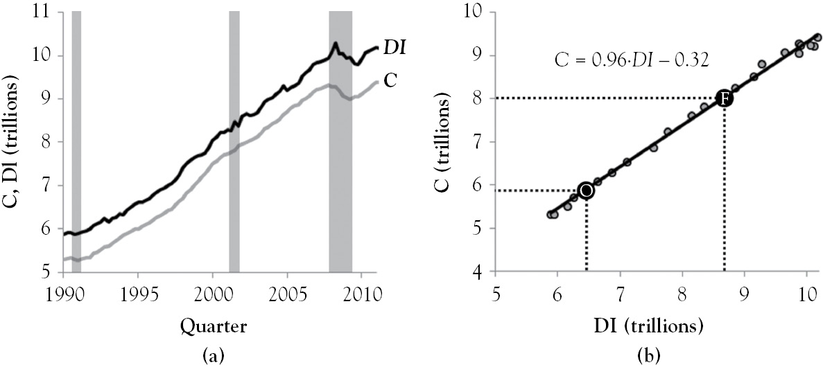
Figure 3.1 Graphs of DI, consumption, and DI versus consumption
The line that fits the scatterplot of consumer expenditure and DI in Figure 3.1b is called the consumption function. From O to F, consumption increases by 2.21 trillion dollars as DI increases by 2.3 trillion dollars. The ratio of the two changes gives the slope of the equation displayed in the figure, 0.96. The slope is called the marginal propensity to consume (mpc). It implies that consumers spend 96 cents of each additional dollar of DI received. The intercept of the consumption function is called autonomous consumption (A) because it models the portion of consumer spending that is independent of DI. The equation in Figure 3.1 gives an empirical estimate of A that equals −0.32. This value implies that consumer spending can be negative and DI can be zero. This is absurd, and results from A being an extrapolated value.3 More generally, the consumption function is
C = A + mpc·DI
In this book, changes to autonomous consumption are used to shift the consumption function. They are caused by exogenous factors4 like consumer wealth (W), expected future consumer income (Ye), the price level (PL), and the real interest rate (r). Because increases in consumer wealth or expected future income, or decreases in the PL or real interest rate raise consumption, simulated autonomous consumption is defined as
A = W + Ye – PL – r
Substituting this into the consumption function gives simulated consumption:
C = [W + Ye – PL – r] + mpc·DI
Simulated consumption can be graphed after values for the mpc (or slope) and the linearly combined autonomous factors (or intercept) are assumed. Suppose that the initial values of consumer wealth, expected future income, the PL, the real interest rate, and the mpc equal 8 trillion dollars, 12 trillion dollars, 14.5 thousand dollars, 3.5 percent, and 0.75, respectively. With the units ignored, substituting the numbers into the equation above yields initial consumption:
C0 = [8 + 12 – 14.5 – 3.5] + 0.75·DI
or
C0 = 2 + 0.75·DI
Simulated consumption shifts when one of the factors in its intercept changes. Because the PL and real rate of interest are subtracted from two other factors in the intercept, a decrease (an increase) in either shifts consumption upward (downward). Since wealth and expected future income are added in the intercept, an increase (a decrease) in either shifts consumption upward (downward). For example, suppose that a decline in consumer sentiment reduces expected future income to 11 trillion dollars. In the equation that follows, the change is highlighted by the number in bold font. Simplifying the result gives final consumption.
C1 = [8 + 11 – 14.5 – 3.5] + 0.75·DI
or
C1 = 1 + 0.75·DI
Final and initial consumption are graphed in Figure 3.2a. Holding DI constant at 8 trillion dollars, the decline in expected future income reduces consumer spending from 8 trillion dollars (at point O) to 7 trillion dollars (at point F).
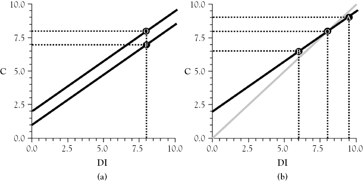
Figure 3.2 Shifts and movements along the consumption function
The consumption model combines the consumption function with a 45-degree line. When the initial consumption line, the black line in Figure 3.2b, crosses the gray 45-degree line, which occurs at point O, consumer savings is zero due to DI equaling consumer spending. In aggregate, consumers save at points along the consumption function that lie below the 45-degree line. For example, at point A consumer savings is 0.5 trillion dollars because consumer expenditure is 9 trillion dollars and DI is 9.5 trillion dollars. At point B, DI exceeds consumer spending, indicating that dissaving occurs at points on the consumption function that lie above the 45-degree line.
Since DI at the macroeconomic level is the difference between real GDP (Y ) and net tax revenue (T ), replacing DI with Y – T in simulated consumption yields:
C = [W + Ye – PL – r] + mpc·(Y – T )
Rearranging this algebraically gives simulated consumer expenditure:
C = [W + Ye – PL – r – mpc·T ] + mpc·Y
Although simulated consumer expenditure is mathematically equivalent to simulated consumption, the two have noteworthy differences. Tax revenue shifts simulated consumer expenditure but not simulated consumption. Simulated consumer expenditure is a function of real GDP, but simulated consumption is a function of DI. To show this, substitute the numbers used to graph initial consumption in Figure 3.2b into simulated consumer expenditure:
C0 = [8 + 12 – 14.5 – 3.5 – 0.75·T ] + 0.75·Y
If initial tax revenue is 3 trillion dollars, initial consumption in terms of real GDP is given by
C0 = [8 + 12 – 14.5 – 3.5 – 0.75 × 3] + 0.75·Y
or
C0 = –0.25 + 0.75·Y
The previously assumed 1-trillion-dollar decline in expected future income, from 12 trillion to 11 trillion dollars, is highlighted by the bold number in the following equation:
C1 = [8 + 11 – 14.5 – 3.5 – 0.75 × 3] + 0.75·Y
Simplifying this gives final consumption in terms of real GDP:
C1 = –1.25 + 0.75·Y
Increases in the real interest rate and PL and a decline in consumer wealth wield similar effects on the intercept of simulated consumer expenditure. Although an increase (a decrease) in net tax revenue does not affect the intercept of simulated consumption, it decreases (increases) the value of simulated consumer expenditure’s intercept.
Net Foreigner Expenditure
The difference in exports (X ), the amount of money foreigners spend on products produced within the boundaries of the United States, and imports (M ), the value of products produced overseas that are purchased within the boundaries of the United States, is called net exports (NX). It is given by
NX = X – M
Since the GDP of other nations determines how much their citizens spend on products produced in the United States, exports are exogenous. Imports, on the other hand, increase as real GDP rises. This is evident in Figure 3.3, the scatterplot of imports versus real GDP for 1990 to 2007.
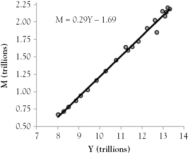
Figure 3.3 Imports (M) versus real GDP (Y)
The black line that fits the data really well in Figure 3.3 is called the import function. It indicates that imports generally rise as real GDP increases. This is due to Americans generally having more income to spend on goods and services produced here and abroad, as real GDP increases. The slope of the line is called the marginal propensity to import (mpm), and is equal to 0.29, according to the equation in Figure 3.3. This value implies that each additional dollar of real GDP raises imports by 29 cents. Although the intercept of the equation in the figure is –1.69, it is assumed to be zero because a nation cannot import products if its GDP is zero. With the mpm undefined, the following gives the simulated import function:
M = mpm·Y
Replacing M in the net exports equation with what it is defined to be above gives simulated net foreigner expenditure:
NX = X – mpm·Y
The above model can be graphed after assuming initial values for exports and the mpm. Suppose their initial values are 2 trillion dollars and 0.25, respectively. With the units ignored, substituting the numbers into simulated net foreigner expenditure gives:
NX = 2 – 0.25·Y
When the above expression is evaluated at real GDP’s value, the result is called the trade balance. If the real GDP is 15 trillion dollars, the trade balance equals –1.75 trillion dollars, which represents a trade deficit. A trade surplus is present when the trade balance is positive.
Aggregate Expenditure
Aggregate expenditure (AE) is the sum of consumer expenditure, net exports, government purchases of goods and services (G ), and investment expenditure (I ):
AE = C + I + G + NX
Substituting simulated consumer expenditure and simulated net foreigner expenditure into the above equation yields
AE = W + Ye – PL – r – mpc ·T + mpc ·Y + I + G + X – mpm ·Y
The left linear combination of variables in bold font is simulated consumer expenditure, while the right linear combination of variables in bold font is simulated net foreigner expenditure. Factoring real GDP gives simulated AE:
AE = [W + Ye – PL – r – mpc·T + I + G + X ] + {mpc – mpm}·Y
The linear combination of variables in the square brackets is simulated AE’s intercept. It models autonomous AE. The expression in the squiggly brackets is AE’s slope.
Using the assumed numerical values in the previous two sections, simulated AE can be graphed after assuming values for government expenditure and investment. Suppose their initial values equal 3 trillion dollars and 2.75 trillion dollars, respectively. With the units ignored, substituting the numbers into simulated AE yields initial AE:
AE0 = [8 + 12 – 14.5 – 3.5 – 0.75 × 3 + 2.75 + 3 + 2] + {0.75 – 0.25}·Y
or
AE0 = 7.5 + 0.5·Y
The AE model combines the AE line with a 45-degree line, which is graphed in Figure 3.4a. The point where AE, the black line in the figure, crosses over the 45-degree line, the gray line, is called the Keynesian equilibrium (point O). At this point, real GDP and AE equal 15 trillion dollars. If the economy is at point B, the aggregate planned expenditure is 13 trillion dollars and the real GDP is 11 trillion dollars. This difference causes an unplanned drop in inventories due to consumers, government, and foreigners buying more goods than they used to. Accelerating inventory depletion rates signal firms that business is picking up. Firms react to higher demand by boosting inventory replenishment rates and ramping up production. This induces a movement along the AE line until the economy reaches the Keynesian equilibrium. At point A, real GDP exceeds aggregate planned expenditure due to consumers, government, and foreigners buying less than they had been buying. This causes an unplanned increase in inventories, signaling firms that business is slowing. Firms respond to lower demand by cutting inventory replenishment rates and production levels. This reduces GDP and pushes the economy toward the Keynesian equilibrium.

Figure 3.4 Movement along and shifts in AE
Simulated AE shifts when one of the factors in its intercept changes. An increase (a decrease) in all these factors but the PL, real interest rate, and net tax revenue shifts AE upward (downward). An increase (a decrease) in the PL, real interest rate, and net tax revenue shifts AE downward (upward). For example, recall the previously assumed 1-trillion-dollar decline in expected future income from 12 trillion to 11 trillion dollars. The change in this factor is highlighted by the bold number in the equation below, which represents final AE after it is simplified.
AE1 = [8 + 11 – 14.5 – 3.5 – 0.75 × 3 + 2.75 + 3 + 2] + {0.75 – 0.25}·Y
or
AE1 = 6.5 + 0.5·Y
Final and initial AE are graphed in Figure 3.4a. The decrease in AE caused by the decline in expected future income reduces the real GDP from 15 trillion dollars (at point O) to 13 trillion dollars (at point F). Multiplying both of these values by the mpm demonstrates that an economic contraction reduces imports. With imports falling from 3.75 trillion to 3.25 trillion dollars and exports being held constant at 2 trillion dollars, the trade deficit falls from 1.75 trillion to 1.25 trillion dollars. The decline in the trade deficit should not be viewed as an “improvement” because it results from an economic contraction.
Fiscal Policy Multipliers
Economists, think-tank policy wonks, executive branch administrators and policy makers, and elected officials who are concerned with short-run fluctuations in unemployment advocate using the federal budget to stabilize the economy. If the 1-trillion-dollar decline in expected future income puts the economy at point F in Figure 3.4a, and potential output is 15 trillion dollars, unemployment is higher than its natural rate. To reduce unemployment and raise real GDP from its present level at point F to its potential at point O, the AE model needs to be shifted back up. A cut in the amount of net tax revenue collected or an increase in government expenditure will increase the value of simulated AE’s intercept, which shifts AE upward and increases real GDP. Deliberate changes to tax rates and government expenditure are called discretionary fiscal policy. At the federal level, it is conducted by Congress and the president. With tax revenue (T) and government expenditure (G) both assumed to be 3 trillion dollars, a cut in taxes or an increase in government expenditure will turn a balanced budget into a budget deficit, which is financed by the U.S. Treasury auctioning securities. Keynesian economics is okay with this because the deficit can be paid off with a budget surplus after the economy returns to full employment.
The government expenditure multiplier is the increase in real GDP that results when government spends an additional dollar. With the economy at point F due to expected future income falling to 11 trillion dollars, suppose that government expenditure is raised by 0.5 trillion dollars to push the economy back toward point O in Figure 3.4b. The increase in government expenditure is highlighted by the bold number in the equation that follows.
AE2 = [8 + 11 – 14.5 – 3.5 – 0.75 × 3 + 2.75 + 3.5 + 2] + {0.75 – 0.25}·Y
or
AE2 = 7 + 0.5·Y
The change in fiscal policy raises the intercept of AE. This shifts AE up to a point along the 45-degree line that is halfway between points O and F. The new line is not shown in Figure 3.4. The shift increases the real GDP from 13 trillion to 14 trillion dollars. Dividing the 1-trillion-dollar increase in real GDP by the 0.5-trillion-dollar increase in government expenditure yields a government expenditure multiplier equal to 2. This value implies that real GDP increases by 2 dollars for each additional dollar government spends.
The tax-cut multiplier is the amount by which GDP rises when taxes are cut by a dollar, holding all else constant. Suppose that the increase in government expenditure is followed by a cut in net tax revenue equal to 0.667 trillion dollars. The new level of net tax revenue equals 2.333 trillion dollars, and is highlighted by the bold number in the equation that follows.
AE3 = [8 + 11 – 14.5 – 3.5 – 0.75 × 2.333 + 2.75 + 3.5 + 2] + {0.75 – 0.25}·Y
or
AE3 = 7 + 0.5·Y
The change in fiscal policy raises the intercept of AE. Together, the back-to-back changes of fiscal policy restore AE’s intercept to its initial value of 7.5. These policy changes shift AE back to its initial level at point O in Figure 3.4b. By itself, the tax cut increases the real GDP from 14 trillion to 15 trillion dollars. Dividing the 1-trillion-dollar rise in real GDP by the 0.667-trillion-dollar tax cut gives a multiplier of −1.5. It implies that real GDP increases by 1.50 dollars for each 1-dollar reduction in taxes. Although the tax-cut multiplier is smaller than the government expenditure multiplier, empirical estimates of tax-cut multipliers tend to be larger than government spending multipliers.5
Although the back-to-back fiscal policies raise real GDP by a total of 2 trillion dollars, they are costly because they result in a budget deficit of 1.167 trillion dollars that is financed with government securities. For this reason, some advocate for a balanced approach. The balanced-budget multiplier is the value by which real GDP increases when government spending and net tax revenue are raised by equal amounts. To demonstrate, suppose that the government responds to the drop in expected future income by raising its expenditure and taxes net of transfers from 3 trillion to 3.5 trillion dollars. Because the previously assumed trillion-dollar decline in expected future income pushed AE to point F in Figure 3.4b, the increases in government expenditure and tax revenue are highlighted by the bold numbers in the equation that follows.
AE2 = [8 + 11 – 14.5 – 3.5 – 0.75 × 3.5 + 2.75 + 3.5 + 2] + {0.75 – 0.25}·Y
or
AE2 = 6.625 + 0.5·Y
The balanced approach barely nudges up AE. It shifts AE from point F in the figure to a new line not shown. This raises real GDP from its dip to 13 trillion dollars (point F) to 13.25 trillion dollars (point not shown). Although the balanced approach seems costless because the budget remains balanced, it is not. Higher tax rates can stifle entrepreneurialism and reduce work effort. The balanced approach is also impotent when the mpc equals 1 because the government expenditure and tax cut multipliers are equal at this value.
The AE model’s fiscal policy multipliers beckon politicians to provide demand when the private sector pulls back. However, the multipliers are overstated because the PL is held constant in the AE model. This is not a concern in Keynesian economics because prices and wages are assumed to be sticky in the short run. This assumption is relaxed in the next chapter.
Aggregate Demand
Aggregate demand (AD) is the relationship between real GDP and the PL, holding all other influences on expenditure plans constant. It is mapped out when a change in the PL shifts the AE line along the 45-degree line, holding all other factors constant. To demonstrate, assume that all of AE’s factors are equal to their assumed initial values. This means that the PL is 14.5 thousand dollars, the economy is at point O in Figure 3.4b, the real GDP demanded is 15 trillion dollars, and simulated AE is given by
AE0 = 7.5 + 0.5·Y
The point corresponding to the initial values of PL and real GDP is labeled “O” in Figure 3.5.
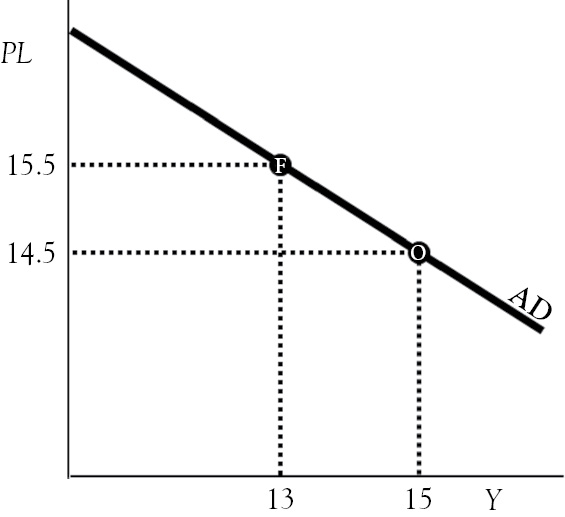
Figure 3.5 Derived aggregate demand
Suppose that the PL increases to 15.5 thousand dollars. This change is illustrated by the bold number in the equation below.
AE1 = [8 + 12 – 15.5 – 3.5 – 0.75 × 3 + 2.75 + 3 + 2] + {0.75 – 0.25}·Y
or
AE1 = 6.5 + 0.5·Y
The increase in the PL shifts the AE line from O to F in Figure 3.4b, which reduces real GDP to 13 trillion dollars. The point corresponding to the final values of PL and real GDP is labeled “F” in Figure 3.5. Drawing a line from O to F in Figure 3.5 traces out AD because the 1-thousand-dollar decline in the PL triggered a 2-trillion-dollar increase in real GDP, holding all other influence on expenditure plans constant.
1 The “Bridge to Nowhere” refers to a proposed bridge connecting Ketchikan, Alaska (population 8,900) with its airport on the Island of Gravina (population 50) at a cost of $320 million (Utt 2005).
2 Using quarterly, seasonally adjusted data FRED from the period 1959–2013, the correlation between total federal government expenditures and civilian employment is 0.91.
3 A regression equation is valid over the range of the dependent variable, DI in this case. The value of the estimated regression intercept in Figure 3.1b is an extrapolated value because the range of DI does not include zero. The error in it is potentially very large since DI’s minimum value is about $6 trillion.
4 An exogenous factor is an independent variable whose value is unaffected by the model.
5 The tax-cut multiplier is estimated at 3 in Romer and Romer (2010), and estimates of the government-spending multiplier are between 0.8 and 1.5 (Ramey 2011).