
Monetary policy is the process by which a nation’s central bank manipulates the supply of money to achieve full employment, maintain a low rate of inflation, or both. In the United States, the central bank is the Fed. Although the Chicago school advocates for central banks to pursue low, steady rates of money growth, the Fed historically has targeted interest rates to fulfill its dual mandate of full employment and low stable inflation.1 Presently, the Fed’s target for unemployment is 5 to 6 percent, and its inflation target is 2 percent.2 For most of its history, the Fed has used the discount rate (id), the reserve requirement ratio (rrr), and its primary policy lever, open market operations, to achieve these objectives. In 2006, Congress gave the Fed an additional monetary tool, paying interest on reserves (ior). Although it was set to begin in 2011,3 due to the 2008 financial crisis, Congress moved its implementation up three years.4 In Operation Twist (Censky 2011), the Fed deviated from purchasing short-term government debt to buying longer term securities to push down long-term interest rates, and spur on home sales and firm investment. Unlike fiscal policy, the Fed can immediately change the supply of money using these tools to counter a recession or fight inflation.
Money
Money takes many forms. It is something that is accepted as payment for products and repayment of debts, legal tender within a country, a store of value, and a standard unit of account. In the absence of money, goods and services are exchanged in a barter system, where individuals directly exchange the surplus from the fruits of their labor. In a barter system, a potato farmer who cannot find anyone looking to trade sacks of potatoes for a plow horse must find someone who needs potatoes and has something horse owners need. Horse owners have a different problem. Unlike a sack of potatoes, a horse cannot be converted into smaller units to be exchanged for an ice cream sundae—unless it is butchered. None of these commodities are a good store of value because ice cream melts, potatoes rot, and horses age.
Money spontaneously arises out of necessity to facilitate exchanges of goods and services.5 The least marketable forms of money were “one by one rejected until at last only a single commodity remained, which was universally employed as a medium of exchange” (Mises 1953). The winner of this contest is divisible, transportable, difficult to counterfeit, and durable. Items ranging from mollusk shells, buckskins, and gold have served as money. In the 1994 movie The Shawshank Redemption, inmates exchanged cigarettes for posters, whiskey, and playing cards. In 2011’s In Time, time is literally money that is used to purchase immortality.
While coins were first minted between 700 and 500 bc (Weatherford 1997), the first paper money, chiao-tzu, was issued in 10th-century Szechwan, China (Lui 1983). It was a bank receipt for iron coins deposited in Szechwan banks. When the Szechwan government took control of this money in 1023, chiao-tzu became the world’s first fiat money, money backed not by commodities but by government decree. In 16th-century London, goldsmiths—artisans who made jewelry out of precious metals—began charging fees for safely storing gold coins.6 The receipts were redeemable to only the depositor unless “or bearer” was printed next to his or her name. In 1694, the Bank of England began issuing receipts named the British Pound. The notes circulated as money because the bearer could redeem them in gold. The notes became fiat money when the United Kingdom abandoned the gold standard in 1931.7
Currently, monetary systems throughout the world use fiat money. In the United States, converting the dollar into fiat money took nearly 40 years. President Franklin Roosevelt essentially ended the gold standard in domestic exchanges and restricted private ownership of gold after signing the Emergency Banking Act of 1933, Executive Order 6102, and the Gold Reserve Act of 1934. President Nixon ended the gold standard in foreign exchanges by issuing Executive Order 11615 in 1971. Meanwhile, “In God We Trust” began appearing on U.S. paper money in 1957.8 Hence, presidents from Roosevelt to Nixon essentially removed the “l” in “gold” on the dollar to slowly transition it from the gold standard to the God standard.
The Market for Money
If holding money or buying bonds are the only stores of wealth,9 the nominal rate of interest determined in the loanable funds market (Figure 5.6b) is the same rate that is determined by equating money demand and supply in the market for money.10 The loanable funds market is ideal for studying discretionary fiscal policy and changes in expected inflation, while the market for money is ideal for understanding the effects of monetary policy; innovation in financial technologies; and changes in income, the PL, and nominal wages.
Money demand is the quantity of money held by the public (Md ) at nominal rate of interest i, holding all else equal.11 The narrowest definition of money is M1. It includes the currency held by the public, which is all paper and coin money held outside of bank vaults. Included in this is the money held in wallets and piggy banks, between couch cushions and car seats, and in businesses’ petty cash drawers. Traveler’s checks, which are not as common as they once were, are included in M1. Although demand deposits include checkable deposits and savings deposits, only checkable deposits are included in M1 because money in checking accounts is easier to access than money in savings accounts. Adding savings deposits and money market mutual funds to M1 yields a broader definition of money called M2.
People and firms demand money because there are benefits to doing so. Although doing so makes it easier to pay for things, the marginal benefit of holding an additional dollar diminishes as the amount held increases. For example, the benefit of holding $2 rather than $1 is much greater than holding an additional dollar when starting with $1,000. Holding the additional dollar is costly because interest is forgone and inflation reduces its buying power. Thus, the nominal rate of interest (i ), the sum of the real interest rate earned on an alternative asset (r) and expected inflation (πe ), is the price of holding money. As it rises, the quantity of money demanded falls. Thus, the Law of Demand holds for money.
The size of money demand’s slope is under debate. On one side of this debate is Irving Fisher with his quantity theory of money, and on the other is Keynes with his liquidity preference theory. Money demand evolved from Fisher’s equation, M · V = Y · PL, where V is money velocity, the number of times one dollar is used to buy products in a given period of time. This equation says the quantity of money multiplied by its velocity equals the nation’s nominal GDP, the product of real GDP (Y ) and the PL. Although Fisher’s view assumes that velocity is constant in the long run and the quantity of money is insensitive to changes in the nominal rate of interest, data suggest that velocity generally slows during recessions and is positively correlated with interest rates.12 Keynes, on the other hand, held that people hold money as a precaution and to conduct daily transactions, and that the quantity of money held for these reasons increases as their incomes rise. He also posited that people hold money for speculative reasons, which would make money demand elastic with respect to the nominal rate of interest.
Friedman’s rework of Fisher’s equation represents a compromise of the competing views. It recognizes current and expected future income as determinants of money demand. This result suggests that the quantity of money demanded is sensitive to changes in the nominal rate of interest. When the current rate is low, the public speculates that future rates will be higher. This makes money more attractive in the present. In addition to recognizing returns from multiple assets and assuming that money and goods are substitutes, the reworked model also allows the return on money to float. This means that money demand is not as sensitive to changes in the nominal rate as Keynes had posited. Figure 6.1a depicts money demand as viewed by Fisher, Keynes, and Friedman. Empirical studies agree that money demand is sensitive to interest rates (Laidler 1993), which is why it is depicted as the downward-sloping line in Figure 6.1b.
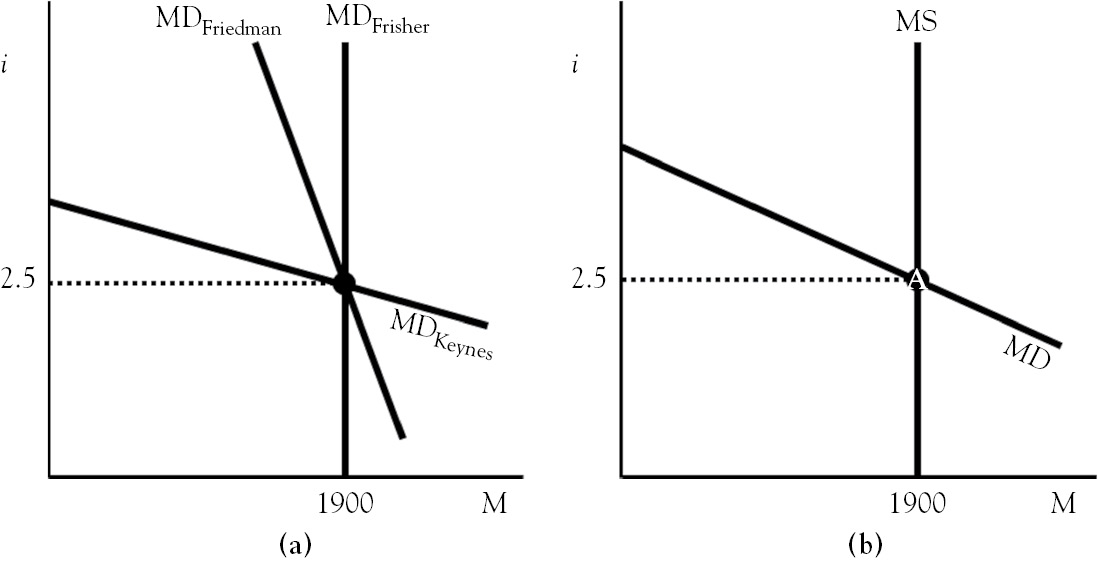
Figure 6.1 Demand for money and the market for money
In addition to money demand depending on nominal interest rate i and real GDP, Fisher’s equation suggests that it also determined by the PL and factors that affect its velocity. His equation implies that the quantity of money demanded will rise by the same percentage as the PL, a view supported by Figure 2.1. Technological innovations such as ATMs, debit cards, and interest-bearing checking accounts increase the velocity of money because they increase the speed at which transactions occur, which in turn increases the demand for money.
The supply of money is the relationship between the quantity of money supplied (Ms) and nominal interest rate i. In Figure 6.1b, the supply of money is perfectly inelastic because the quantity of money supplied is determined by bank lending and the Fed’s open market operations.
The equilibrium in the market for money occurs at the intersection of money demand and money supply. The nominal rate of interest adjusts to make the quantities of money demanded and supplied equal. When the nominal interest rate is above its equilibrium, the quantity of money supplied exceeds the quantity of money demanded, which means people are holding too much money. To rid themselves of it, they buy financial assets like bonds. This increases the demand for bonds, which increases their prices. Since bond prices and interest rates are negatively related, the nominal interest rate falls until the quantities of money supplied and money demanded equate (at point A in Figure 6.1b). When the quantity of money demanded exceeds the quantity supplied, the interest rate is below its equilibrium. This means that people are holding too little money and seek more by selling bonds. This reduces bond prices and pushes nominal interest rates up until the quantities of money demanded and supplied are equal.
Banking
The modern U.S. bank is a financial intermediary that accepts deposits from savers and lends money to borrowers. It evolved from 16th-century London goldsmiths. Goldsmiths had a history of safely storing gold coins, which was the medium of exchange at the time. Table 6.1a shows a hypothetical T-account for a 16th-century London goldsmith, whose first gold coin deposit was made by John for the amount of 200 coins. Notice that the amount is considered an asset and a liability as it is listed on both sides of the T-account. The value on the left is called reserves because the gold coins are being reserved for the depositor. The value on the right is called demand deposits because the depositor can demand his gold at any time.
Table 6.1 Sixteenth century London goldsmith T-accounts
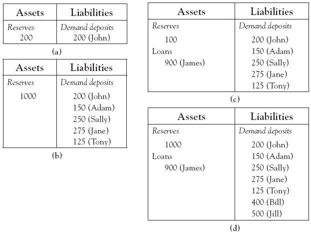
Storing gold is profitable because John, whose employer pays him in gold coins, is willing to pay to have it safely kept by the goldsmith. Storing it in one’s home or carrying it on one’s person is risky, and depositing it at the goldsmith is not too inconvenient because it is located near his village’s ale house and shops. Table 6.1b shows what happens when word spreads of the goldsmith’s ability to safely store John’s gold. Others deposit their gold in the goldsmith’s safe, raising his assets and liabilities to 1,000 coins. As the proceeds from storage fees pile up, the goldsmith’s wealth grows, and storing gold becomes his primary business.
After observing the goldsmith’s growing affluence, James inquires about borrowing some of the gold that is sitting idle in the goldsmith’s safe to turn his alehouse into an inn. The goldsmith will accommodate the request if he believes depositors will keep their coins in his safe for the desired length of the loan, the inn will be profitable, and James is willing and able to pay back the principal, the borrowed gold coins, and interest, compensation for accepting credit risk.
Because the gold coins are the property of others, lending them to others could be viewed as unscrupulous. To overcome this, the goldsmith offers to pay depositors interest. If the net interest margin, the difference between the rate borrowers pay and the rate depositors require, is negative, the goldsmith makes a loss. Even if the net interest margin is positive, the goldsmith may hesitate to make the loan because demand deposits can be withdrawn at any time. The goldsmith, however, can protect himself by offering higher interest to depositors who agree to keep gold coins in his safe for a given length of time, say, the life of the loan. Such a deposit is called a time deposit. Although it comes with a lower net interest margin, time deposits safely securitize the loan. This is important because government backstops (e.g., discount loans, Federal Deposit Insurance Corporation, bailouts for too-big-to-fail banks, and Fannie Mae and Freddie Mac) did not exist at the time.
Table 6.1c shows the immediate effect of the goldsmith agreeing to give James a one-year interest-bearing loan of 900 gold coins. The goldsmith’s reserves drop to 100 coins because 900 have been removed from the goldsmith’s safe and handed over to James. After James pays 500 gold coins to Jill for building materials and 400 to Bill for his labor, the borrowed gold coins get deposited back into the goldsmith’s safe, which is shown in Table 6.1d. Notice that even though the total number of coins in the safe is only 1,000, demand deposits increased to 1,900. The ratio of these two numbers, called the reserves ratio, indicates that only 53 percent of the goldsmith’s reserves are backing demand deposits.
A self-imposed reserves ratio is called the desired reserves ratio. Its value is determined over time, via trial and error. During the process of making additional loans and accepting more gold coin deposits, suppose the goldsmith discovers a reserves ratio of 0.2 is enough to balance outflows (gold withdrawals and gold payments from new loans) with inflows (new gold deposits and loan payoffs in gold) under normal economic conditions. The goldsmith will make loans until demand deposits swell to five times the number of gold coins held in reserve. This is shown in Table 6.2a. With 10,000 coins physically held in the goldsmith’s safe, he comfortably makes loans worth 40,000 coins to villagers. This inflates the value of demand deposits, which are worth 50,000 coins. The goldsmith also discovers that the paper receipts he has issued are circulating in the local economy. As long as he always redeems the receipts in gold coins, villagers consider them money because they are as good as gold. The coin receipts are increasingly preferred to gold coins because they can be folded, and their use eliminates trips to the goldsmith.
Table 6.2 Banking before and after reserve requirements were imposed

The system described above is called fractional reserve banking because reserves are a fraction of demand deposits. Such a system is inherently risky because bank profits increase as the reserves ratio falls. Consider the goldsmith example above. As his banking operations expand, he works less and less as an artisan and increasingly more as a banker. Balancing his T-account and reviewing loan applications is time consuming but is necessary to ensure a desired reserves ratio of 0.2. If the economy over performs for a longer-than-expected period of time, it may give him a false sense of security. As such, he may decide that a desired reserves ratio of 0.1 is fine. At that ratio, only 10,000 coins are backing 100,000 in demand deposits. This allows him to make loans worth 90,000 in coins. At 5 percent interest, this increases the interest payments he receives by 125 percent. His new position is more profitable but riskier. For example, an unexpected event like the Little Ice Age (1560 to 1850) that killed English vineyards wipes him out. A collapse in winery revenues slows the number of gold coins being deposited and increases the number of coins being withdrawn as vineyard workers migrate to southern France. After workers withdraw 10,000 coins, the remaining 90,000 receipts for coins are worthless.
In the United States’ fractional reserve banking system, the Fed, currently imposes a required reserves ratio (rrr) of 0.1 on checkable demand deposits (D). This makes banks’ T-accounts slightly different from the goldsmith’s. Reserves and loans are still listed on the asset side, but reserves are split into required reserves and excess reserves. Table 6.2b illustrates this difference. For purposes of comparison, the table assumes that the bank’s inflows and outflows are balanced, with a desired reserves ratio of 0.2. This means that the bank voluntarily lends out all but $10,000 of the $50,000 in checkable demand deposits. The bank’s outstanding loans of $40,000 are split among loans to government (in the form of securities), consumers (for homes and autos), and businesses. With bank reserves equaling $10,000 and a rrr of 0.1, the bank’s required reserves and excess reserves each equals $5,000.
Multiple Deposit Creation
While lending in the goldsmith example above increased the supply of money in a few steps, infinitely many progressively smaller loans are made in the simple multiple deposit creation model found in most textbooks. In the simplest version of this model, banks do not hold excess reserves, and no one holds currency. Suppose Fred deposits $1,000 he found buried in his backyard. At the moment Fred finds the money, the money supply increases by $1,000. With a rrr of 0.1, Fred’s bank must hold $100 of the $1,000 deposit in reserve. This allows the bank to lend George $900 to buy a TV. The money supply increases by $900 the moment the bank deposits the loan into George’s checking account. If George immediately swipes his debit card at Biggie-Mart to buy a $900 TV, the bank moves $900 from George’s account to Biggie-Mart’s. At that moment, the money supply does not change because moving money from one depositor to another is like moving sand from one side of a beach to the other. Because the bank is required to hold $90 of the $900 deposit as reserves, it can lend the rest to Carol. At the moment the $810 is deposited in her checking account, the money supply increases by that amount in a second round of lending. Lending money into existence continues. It increases by $729 in the third round of lending, by $0.03 in the 100th round, by almost 0 in round 150, and exactly 0 after infinitely many rounds. Fred’s $1,000 deposit raises demand deposits to $1,900 after the first round, to $2,710 after the second, to $3,439 after third, to $9,999.76 after the 100th, almost $10,000 after the 150th, and exactly $10,000 after infinitely many. Because the increase in demand deposits equals Fred’s $1,000 cash injection divided by the rrr, the inverse of the rrr is the simple money multiplier.
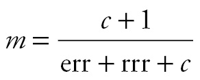
The money multiplier is the increase in money circulating in the economy for each dollar the Fed adds to reserves. It is the inverse of the rrr, provided no one holds cash and banks convert all excess reserves into loans. Individuals and firms hold currency for some transactions, which means that borrowers tend to convert a small portion of checkable deposits into currency. This is called the currency ratio (c), and is equal to the ratio of currency (c) to checkable demand deposits. Banks also hold cash called excess reserves (Re). Some banks hold more than others. The ratio of excess reserves to checkable deposits is called the excess reserves ratio (err). When banks and others hold cash, the money multiplier is given by13
If the err equals 0.1, the rrr is 0.1, and currency drain is 0.05, the money multiplier is 4.2. This means that, for each dollar the Fed adds to reserves, the money supply increases by $4.20. If the Fed removes a dollar instead, the money circulating in the economy falls by $4.20. Thus, banks can lend money into and out of existence.
Unforeseen events and economic cycles affect the potency of the Fed’s injections and withdrawals of reserves. A shock to the economy caused by a terrorist attack or a natural disaster can induce depositors to convert demand deposits into cash and banks to hold more excess reserves. If the currency ratio and err rise to 0.4 and 0.8, respectively, the money multiplier dips to 1.08 and the potency of monetary policy declines by 74 percent. When the economy grows robustly, banks tend to make more loans. This pushes the err toward zero, and raises the money multiplier and the potency of monetary policy.
The Federal Reserve System
The Fed was established in 1913 and is charged with regulating banks, supervising the payments system, setting reserve requirements, and being a lender of last resort in times of financial emergencies. The system is comprised of 12 district banks and is managed by the Board of Governors (BOG). The seven members of the BOG are appointed by the president and confirmed by the Senate. Each member serves for 14 years, cannot serve more than one complete term, and cannot be removed for political reasons. Staggering members’ terms every two years provides a modicum of certainty to markets, while term length hinders political influence from elected officials. Political influence is further limited by the Fed financing its operations from check-clearing fees and interest collected on loans to commercial banks and government.
Although independence allows the board to pursue policies that are “best” for the economy—not the president or Congress—this autonomy is somewhat limited. Every four years the president appoints and the Senate confirms a member of the BOG to serve as its chair. Members of the BOG also testify before Congressional committees and meet or work with the Council of Economic Advisors, Treasury, Federal Advisory Council, Federal Deposit Insurance Corporation, and others. The Fed submits biannual reports to Congress and is subject to annual Government Accountability Office audits.
The Federal Open Market Committee (FOMC) sets monetary policy for the Fed. All seven BOG members, the president of the New York Federal Reserve Bank, and four other District Bank presidents sit on the FOMC. The board’s chair also heads the FOMC, which meets every sixth Tuesday. Monetary policy is set in these meetings.
The Federal Funds Market
To keep unemployment and inflation in check, the Fed controls the quantity of reserves circulating in the federal funds market using the discount rate, the reserve requirement ratio, open market operations, and interest on reserves. In the absence of discount lending and interest payments on reserves, the market for money and the federal funds market look very similar. In Figure 6.2a, reserves supply (RS) is perfectly inelastic, and reserves demand (RD) slopes downward. The federal funds market is in equilibrium at point H, reserves equal 80 billion dollars, and the federal funds rate is 1.5 percent, which is less than the interest rate shown in Figure 6.1b.
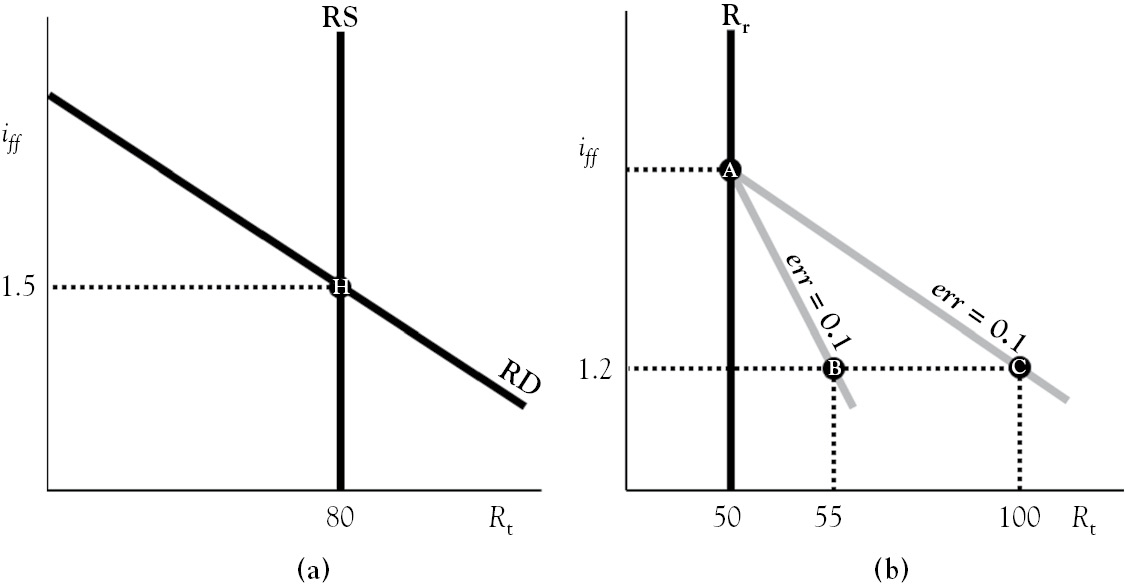
Figure 6.2 Historical mode in the federal funds market and derivation of reserves demand
The quantity of reserves demanded is the sum of required reserves and the quantity of excess reserves demanded. Required reserves is total checkable demand deposits in the banking system multiplied by the rrr. For example, when the rrr is 0.1 and checkable demand deposits equal 500 billion dollars, the quantity of required reserves is 50 billion dollars.
The quantity of excess reserves demanded depends on many factors. Early macroeconomists attributed high excess reserves during the Great Depression to too few worthy loan opportunities (Frost 1971). This was perhaps due to poor economic growth or New Deal wage and price controls interfering with pricing signals that may have stifled innovation and entrepreneurialism. The quantity of excess reserves demanded varies inversely with deposit potential (Frost 1971), the maximum deposit level that can be maintained with no excess reserves and no vault cash. It declines in real GDP because, as the economy expands, default risk falls and consumer and business lending rises. It varies with overdraft fees the Fed charges banks for not covering daily transactions (Edwards 1997), and jumps up when the Fed adjusts the rrr (up or down) due to heightened uncertainty (Dow 2001). Excess reserves spike following bank panics (Friedman and Schwartz 1963) that are caused by natural disasters, acts of war, or economic shocks at home or abroad. Because the above factors are assumed constant within a given day, they are lumped into shock s.
In addition to the aforementioned factors, the quantity of excess reserves demanded depends on the federal funds rate (if f ). The relationship between these two variables is negative (Poole 1968), and, for the moment, is assumed to be the following simple relationship.
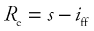
Holding excess reserves insures against withdrawals, but doing so has a cost. The cost increases as the federal funds rate rises. When a bank holds excess reserves, it foregoes the opportunity to lend them to another bank needing to meet its reserve requirement. Thus, holding excess reserves is analogous to adding collision and comprehensive coverage to a car’s liability insurance policy.
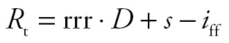
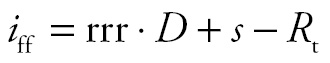
Adding required reserves (rrr·D) and excess reserves (s – iff ) gives total reserves (Rt):
Solving it for the federal funds rate yields reserves demand:
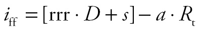
Although the equation suggests that reserves demand has a slope of −1, Figure 6.2b suggests that the slope is related to the err. At all three points in the figure, required reserves total 50 billion dollars. This is due to banks being required to keep 10 percent of their checkable deposits, 500 billion dollars in this example, on reserve. At point A, banks hold zero excess reserves because the federal funds rate is relatively high. The quantity of excess reserves is 5 billion dollars at point B but is 50 billion dollars at point C. With checkable deposits totaling 500 billion dollars, the err is zero at point A, 0.01 at point B, and 0.1 at point C. Thus, the line in the figure steepens as the err rises. Accounting for this in the equation above is accomplished by replacing slope –1 with –a, which gives simulated reserves demand:
For simulation purposes, a is scaled between 0 and 1. It models banks’ aversion to holding excess reserves because it is inversely related to the err. Suppose slope a equals 0.8 and shock s equals 15.5. With a rrr of 0.1 and checkable deposits equal to 500 billion dollars, the equation for reserves demand is given by
iff = [0.1 × 500 + 15.5] – 0.8·Rt
or
iff = 65.5 – 0.8·Rt
The graph of this equation passes through point H in Figure 6.2a.
Reserves demand shifts if the reserve requirement ratio, checkable demand deposits, or a bank panic occurs. For example, suppose a bank panic at a large international bank causes shock s to jump from 15.5 to 16.5. This change is highlighted by the number in bold font below.
iff = [0.1 × 500 + 16.5] – 0.8·Rt
or
iff = 66.5 – 0.8·Rt
The graph of this equation would lie to the right of the black line in Figure 6.2a, if shown.
Prior to 2003, the discount rate was set below the federal funds rate. This situation is called historic mode. When the federal funds market is in historic mode there is an incentive for banks to borrow from the Fed instead of other banks. The Fed deterred this by requiring banks to exhaust all other credit sources and justify their credit needs, and audited banks that abused the discount window. Ninety years after its founding, the Fed began setting the discount rate 1 percentage point above its target for the federal funds rate. This kinks reserves supply at point K in Figure 6.3a.
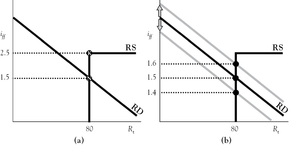
Figure 6.3 Normal mode in the federal funds market
The kinked simulated reserves supply curve has two parts. The vertical part is the sum of nonborrowed reserves (Rn) and borrowed reserves (Rb), while the horizontal section is the nonbinding price ceiling known as the discount rate. Suppose nonborrowed and borrowed reserves are 0 and 80 billion dollars, respectively. With the sum of the two equal to 80 billion dollars, the vertical section of reserves supply is the vertical line segment in Figure 6.3a that ends at point K. With the discount rate at 2.5 percent, the horizontal section of reserves supply is the horizontal line segment that starts at point K and continues to the right.
When reserves demand intersects the vertical section of supply, as it does at point N, the federal funds market is in normal mode. The federal funds market remains in normal mode as long as reserves demand crosses the vertical section of reserves supply. Normal fluctuations in real GDP vary with real incomes, causing checkable deposits to fluctuate. According to the following equation, fluctuations in checkable deposits causes the intercept of simulated reserves demand to vary and reserves demand to bounce.
These oscillations are demonstrated in Figure 6.3b. They cause the federal funds rate to cycle between 1.4 percent and 1.6 percent. As this happens, the federal funds market remains in normal mode.
A bank panic has two effects. Demand flattens as aversion to holding excess reserves (a) falls. After demand flattens, it shifts rightward because the panic causes s to jump in value.
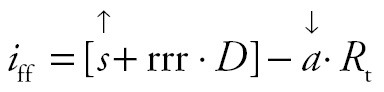
Figure 6.4a shows that the bank panic puts the federal funds market in emergency mode, a situation where the equilibrium (point E) is on the flat section of reserves supply. At this point, banks demand 90 billion dollars but only 80 billion dollars is supplied. If the Fed, the lender of last resort, does not lend banks the difference, the federal funds rate rises to 2.6 percent. The Fed averts this by making 10 billion dollars in discount loans. This raises borrowed reserves to 10 billion dollars, and total reserves to 90 billion dollars.
Figure 6.4 Emergency mode in the federal funds market and adjustment of the rrr
Monetary Policy
The Fed currently regulates the federal funds market to maintain unemployment between 5 percent and 6 percent and inflation near 2 percent. Because the Fed cannot directly control unemployment, inflation, and economic growth, it targets money growth or interest rates by injecting or pulling reserves from the federal funds market. Because monetarists like Milton Friedman advocate for low, steady, stable money growth, targeting money aligns with the classical school and its focus on the long run. Targeting interest rates is embraced by Keynesians because a reduction in interest rates boosts AD via greater investment. Austrian economists would consider targeting money the lesser of the two evils, because artificially low interest rates lead to malinvestment and speculative economic bubbles.14 The Fed uses several tools to target interest rates or money growth.
Discount lending is an emergency monetary policy tool. After a 2003 policy change, the Fed sets the discount rate one percentage point above its target for the federal funds rate. Figure 6.4b shows what happens when the discount rate is adjusted between 2.5 percent and 3.0 percent. The figure shows that small adjusts to the discount rate have no effect on reserves or the federal funds rate.
Adjusting the rrr has an effect similar to that of a bank panic. Raising it shifts reserves demand outward. Because the change injects uncertainty into the banking system, shock s spikes and aversion to holding excess reserves (a) falls.
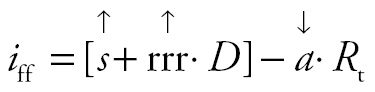
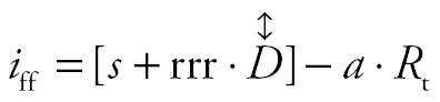
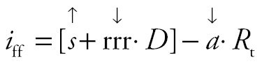
The three effects make predictions difficult because they flatten and shift demand outward, as shown in Figure 6.4a. Although the figure shows reserves rising, the money supply falls from point A to point B in Figure 6.5a. A decline in the money supply increases the nominal rate of interest and the real interest rate (r), if expected inflation does not change. This dampens private investment (I ), and strengthens the dollar, which reduces exports (X ). The effects of the changes in these variables are modeled by arrows in the equation below.

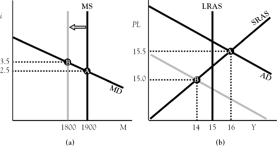
Figure 6.5 Effects of adjusting the rrr
In Figure 6.5b, the net effect of hiking the rrr decreases AD from the inflationary gap at point A to the recessionary gap at point B, reduces real GDP and the PL, and raises unemployment above its natural rate.
If the Fed decides to lower the rrr instead, the uncertainty triggered by this change in policy causes shock s to spike up and banks’ aversion to holding excess reserves to fall:
Although less aversion to holding excess reserves flattens reserves demand, the net effect of shock s and cutting the rrr is ambiguous. After flattening, reserves demand shifts up if shock s swamps the rrr effect, but shifts down if shock s is swamped by the rrr effect. This unpredictability is perhaps why the Fed has not adjusted the rrr since 1992.15
It appears that the Keynesian school has won the what-to-target debate, because the Fed has historically targeted interest rates. Interest rates are adjusted when the Fed sells and buys Treasuries. These transactions are called open market operations, which were discovered accidentally. During World War I, Federal Reserve District Banks were earning substantial interest on loans made to banks. The deflationary recession of 1920 to 1921 allowed banks to pay off most of these loans. Left with dwindling streams of income, District Banks began buying securities from banks to cover their expenses. The purchases, uncoordinated at the time, led to an enormous expansion in the money supply. In response to that discovery, the Fed formed what is now known as the FOMC in 1922. Due to its proximity to world financial markets, the New York Federal Reserve Bank conducts open market operations on behalf of the FOMC.
Suppose the Fed decides to lower its target for the federal funds rate from 1.5 percent to 0.25 percent to stimulate the economy out of a recessionary gap. To do this, it buys securities from banks in open market purchases. In Figure 6.6a, the 12.5-billion-dollar open market purchase increases the quantity of nonborrowed reserves by the same amount, and pushes the federal funds from 1.5 percent (point A) to its new target of 0.25 percent (point B). In accordance with its 2003 policy change, the Fed lowers the discount rate from 2.5 to 1.25 percent. If the money multiplier is 4.2, the 12.5-billion-dollar increase in reserves is expected to increase the money supply by 52.5 billion dollars and reduce the nominal interest rate to 1.25 percent, according to Figure 6.6b.
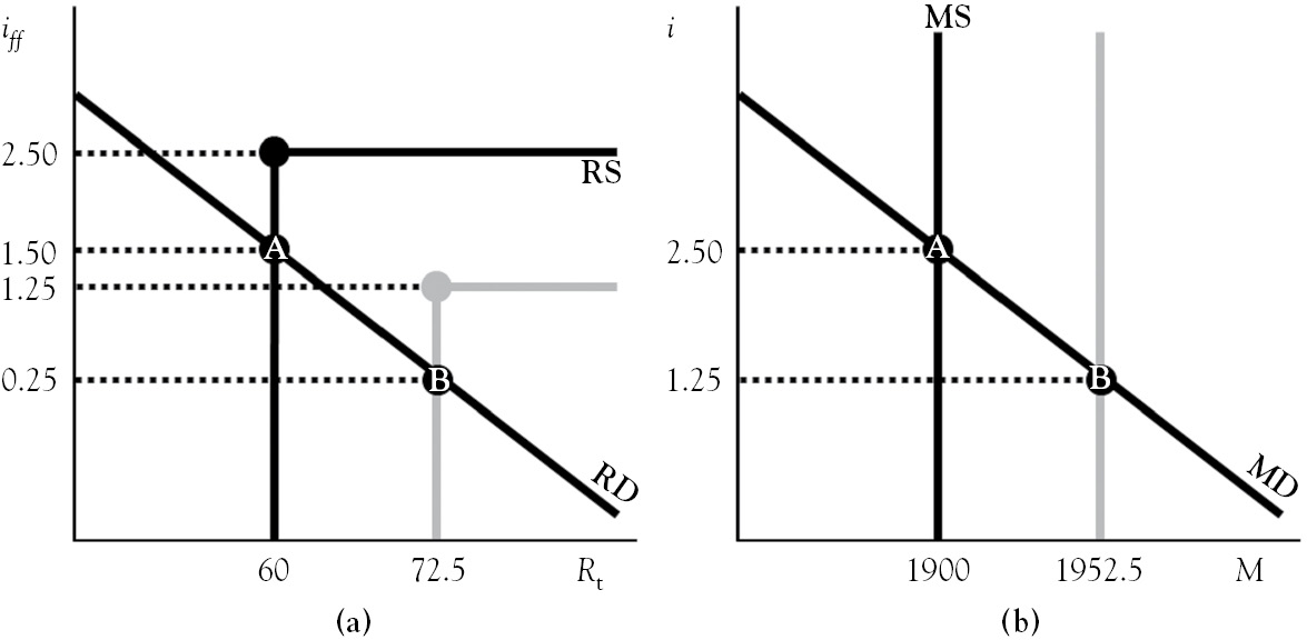
Figure 6.6 Open market purchase and its effect on the market for money
The open market purchase affects AD in several ways. If expected inflation remains unchanged, the decline in the nominal interest rate decreases the real rate (r). This boosts private investment (I ), and lowers the value of the dollar, which raises exports (X ).

Collectively, these effects shift AD from A to B in Figure 6.7a. This closes the output gap, reduces unemployment, and causes the PL to rise to 16.5 thousand dollars.
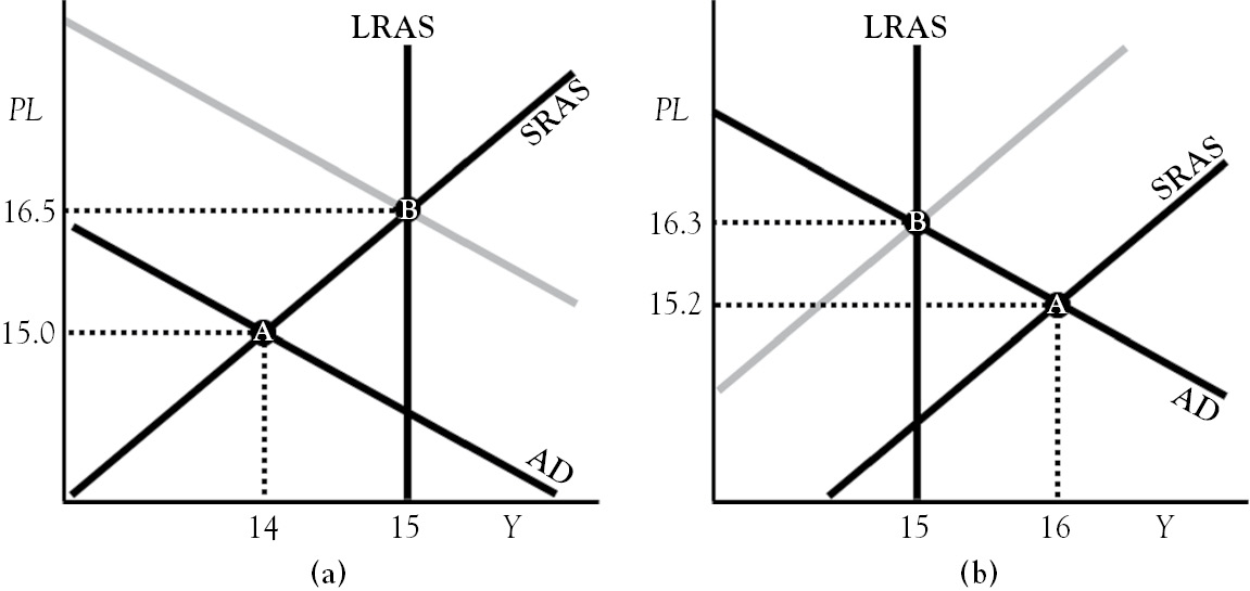
Figure 6.7 The effects of open market operations on the aggregate market model
An open market sale is used to close an inflationary gap, like the one at point A in Figure 6.7b. It involves the Fed selling previously purchased Treasuries to banks. In Figure 6.8a, the federal funds rate is increased from 1.2 percent to 1.5 percent by a sale that reduces the quantity of reserves from 65 billion to 60 billion dollars. If the money multiplier is 4.2, the 5-billion-dollar decrease in reserves is expected to decrease the money supply by 21 billion dollars. The resulting increase in the nominal interest rate raises real rates, if expected inflation is stable. Higher interest rates reduce private investment. The higher interest rates also increase the value of the dollar as foreign investors use dollars to buy U.S. securities. The appreciating dollar makes American goods more expensive overseas, which reduces U.S. exports. These effects shift AD from A to B in Figure 6.7b, which closes the output gap and raises unemployment and the PL.
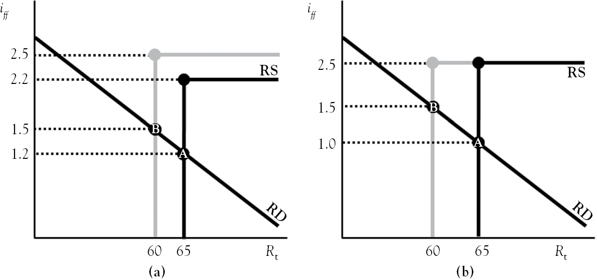
Figure 6.8 Open market sales
Oscillations in reserves are normal. They are caused by fluctuations in checkable deposits that are due to economic cycles. At point A in Figure 6.8b, one such fluctuation has the federal funds rate at 1 percent, which is below its target of 1.5 percent. To push the rate back up to its 1.5 percent target, the figure shows the Fed conducting an open market sale of 5 billion dollars. However, in doing this, the money supply falls by 21 billion dollars, assuming that the money multiplier is 4.2. Although only one open market operation is used in this example, the New York Federal Reserve Bank constantly sells and buys Treasuries to keep the federal funds rate near its target. In doing this, the Fed causes money supply variations via multiple deposit creation. If instead the Fed targets money, it injects or withdraws reserves to keep money growing at a slow steady pace. As this is going on, interest rates fluctuate due to oscillations in reserves demand. Thus, the Fed can target interest rates or money growth—not both.
Near the beginning of the Fed’s rescue of the financial system in 2008, it began paying interest on reserves (ior), which is a price floor on the federal funds rate. From the 2008 collapse of Lehman Brothers to the spring of 2010, the Fed’s holdings of securities rose by roughly 1.7 trillion dollars (Zumbrun 2013). If the Fed had not begun paying interest on reserves, the example depicted in Figure 6.9a shows that its unprecedented purchases of mortgage-backed securities and Treasuries would have resulted in a negative federal funds rate. Paying interest on reserves kinks reserves demand at D because banks prefer earning that rate for the reserves they hold at the Fed rather than a negative rate they would have earned had they lent their reserves to other banks. The federal funds market is in crisis mode when it equilibrates at point C in Figure 6.9b.
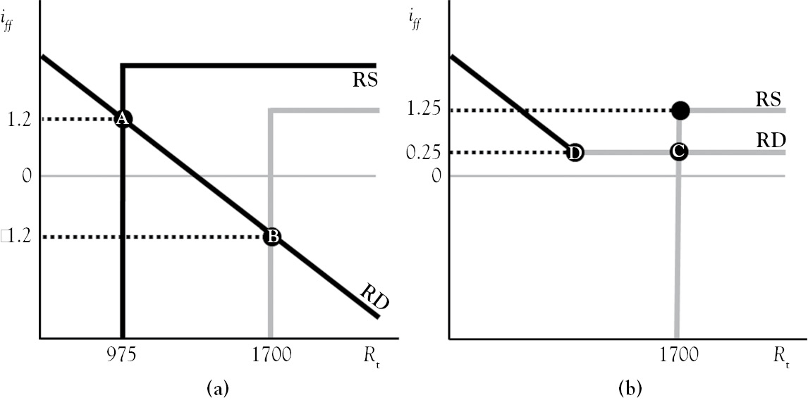
Figure 6.9 Crisis mode in the federal funds market
Crisis mode has several interesting consequences. It allows the Fed to buy and sell securities without affecting changes in the federal funds rate. This is so because reserves supply slides left and right as the Fed conducts open market operations. Kinking reserves demand at a near zero interest rate also allows the Fed to buy or sell securities without affecting changes in the money supply. According to Frost (1971), the federal funds market is in a liquidity trap when reserves demand is very elastic and the federal funds rate is below 0.5 percent. The flat section of reserves demand in Figure 6.9 mimics the elastic section of the reserve demand curve Frost observed.
Monetary Policy in Practice
As demonstrated earlier, the Fed can target interest rates or money growth, not both. If it targets interest rates, it uses open market sales and purchases to keep a fluctuating federal funds rate near its target. This causes the money supply to contract and expand via multiple deposit creation. On the other hand, the normal ebbs and flows of money demand and reserves demand can cause interest rates to fluctuate if the Fed follows Milton Friedman’s monetary rule: low and steady money growth. In theory, this can cause real GDP to cycle around potential output as AD undulates around LRAS and SRAS. Since news reports of accelerating inflation and persistently high unemployment pull on the heartstrings of voters, money targeting is the harder sell, politically.
The Fed has mostly targeted interest rates in the post-World War II era. Between 1952 and 1969, the Fed explicitly targeted interest rates. Figure 6.10a indicates that annual M2 growth dropped to about 2 percent during the recessions at the beginning and end of the 1960s. In between the two recessions, money growth increased by a factor of 4. This results from the Fed conducting substantial open market purchases to keep interest rates low for an extended period of time during a long economic expansion. Between the two recessions, each dollar that the Fed injected into reserves raised the money supply by about $2.74, according to Figure 6.10b.16 The resulting high rate of money growth, which was near 8 percent for most of the decade, fans inflationary flames. Although inflation floated steadily near 1.3 percent for the 1959 to 1964 period, it accelerated from 1.1 percent in the third quarter of 1964 to 6.2 percent by first quarter of 1970. This is one of the consequences Friedman (1968) foresaw when the Fed tries to keep interest rates too low for too long.
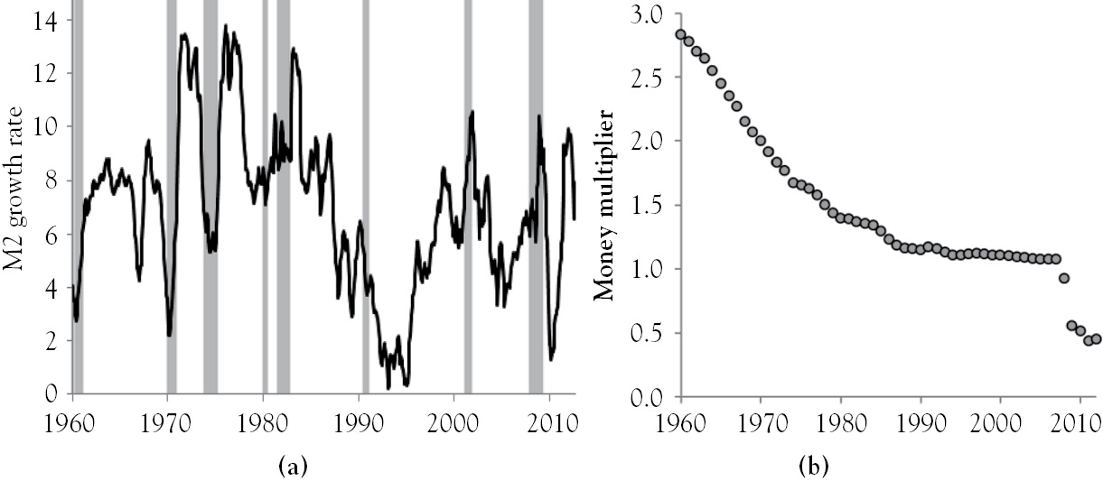
Figure 6.10 Graphs of M2 growth and the money multiplier
Although Friedman’s monetary rule was the stated policy of the Fed in 1970 when Arthur Burns became its chair, it continued to target interest rates. This is evident in Figure 6.10a. Money growth was more volatile during the 1970s than it had been during the previous decade. Money growth peaked near 14 percent during expansions and fell to 6 percent during the recession of the mid-1970s. The procyclical monetary policy caused inflation expectations to fluctuate wildly, which slayed the Phillips curve and spurred on an inflation spiral that Paul Volcker was charged with tackling when he was appointed to head the Fed in 1979.
Unlike his predecessors, Volcker’s monetary policy was countercyclical, which is evident in Figure 6.10a. His targeting of bank reserves yielded relatively low volatility in money growth that trended upward during the recession of the early 1980s. Thereafter, money growth was a bit more volatile. The rate of growth in money generally fell from its high of nearly 13 percent at the beginning of the 1980s to 0.3 percent by the second month of 1993. The high federal funds rate at the beginning of the 1980s is associated with persistently high unemployment. This was not unintended because the augmented Phillips curve in Figure 2.9b predicts that inflation will fall by two percentage points per year when unemployment remains elevated at around 9 percent. The high persistent unemployment lowered inflation from 13 percent in 1980 to 11 percent in a year, 9 percent in 2 years, and 4 percent by 1984.
After Alan Greenspan was appointed to chair the Fed in 1987, the Fed began targeting interest rates again. Near the end of 1992, the Fed set the federal funds rate to 3 percent, where it remained until early 1994. Figure 6.11a shows that this was followed by a precipitous decline in unemployment. The Fed responded by raising the federal funds rate to 6 percent in 1995 and held it there until 1998. However, as unemployment continued to fall, the Fed bumped the funds rate up to 6.5 percent. A sharp rise in unemployment ensued, which preceded the 2001 recession. To right the ship, the Fed dropped the funds rate to 2 percent near the end of 2001. Unemployment stabilized, but another marked decline began. In 2004, as unemployment continued to fall, the Fed steadily raised the federal funds rate from 1 percent to 5.25 percent. About halfway through that process, Ben Bernanke was picked to head the Fed. After bottoming out a few months prior to the start of the Great Recession, unemployment exploded and crested above 10 percent in 2009. The Fed responded to this by essentially zeroing the federal funds rate with the trillions of reserves it injected into the banking system.
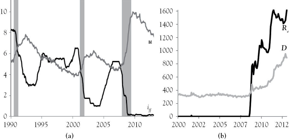
Figure 6.11 Graphs of iff, u, Re, and D
With banks currently holding trillions of dollars in excess reserves (see Figure 6.11b), and the Fed owning trillions of dollars in securities, the seeds of future inflation have been sowed. Although the persistent output gap (see Figure 2.7a) and continued weakness in labor markets is keeping inflation at bay, robust economic growth at some point in the future will make banks more optimistic and more averse to holding excess reserves. The excess reserves would result in a trillion or so of additional dollars circulating in the economy, if the money multiplier returns to its pre-Great Recession level of about 1.1 (see Figure 6.10b). If the money multiplier returns to its President Kennedy-era level, excess reserves could burst into 4 trillion dollars or more in additional money in circulation. To keep the inflation genie in the bottle, the Fed will have to raise interest on reserves while selling off some of the securities it owns. However, if these securities are liquidated too quickly, the Fed could flood the economy with trillions of dollars. Because banks can buy securities from whomever they want, the Fed and the U.S. Treasury would be competing for the same buyers. With Figure 2.1 indicating a nearly one-for-one relationship between inflation and money growth, future inflation could be substantial.
History is littered with examples of hyperinflation. Larry Allen’s (2009) The Encyclopedia of Money discusses 21 such examples. Prior to the 1917 Bolshevik Revolution, hyperinflation resulted in prices rising two to three times faster than wages. After the Bolsheviks took power, hyperinflation exploded from 92,300 percent for the period 1913 to 1919 to 64,823,000,000 percent for the period 1913 to 1923. In 1914, there were 6.3 billion marks circulating in the German economy, but by 1923, there were 17,393 billion. A newspaper costing one mark in May 1922 cost 1,000 marks 16 months later and 70 million marks a year-and-a-half later. Erich Maria Remarque’s The Black Obelisk describes how hyperinflation adversely affected the German people, writing: “Workmen are given their pay twice a day now—in the morning and in the afternoon, with a recess of a half-hour each time so that they can rush out and buy things—for if they waited a few hours the value of their money would drop.” Customers rolled wheelbarrows full of money to the grocery store, the cost of meals at restaurants were negotiated before orders were placed, and paper money was baled like hay to heat one’s home. Although it took about four days for prices to double with inflation at its worst in Germany, prices doubled in 33.6, 24.7, and 15.6 hours in 1994 Yugoslavia, 2008 Zimbabwe, and 1946 Hungary, respectively (Hanke 2009).
1 Congress restated the Federal Reserve’s objectives when it amended The Federal Reserve Act in 1977.
3 See the Financial Services Regulatory Relief Act of 2006 at www.gpo.gov
4 See the Emergency Economic Stabilization Act of 2008 at www.gpo.gov
5 “When the inhabitants of one country became more dependent on those of another, and they imported what they needed, and exported what they had too much of, money necessarily came into use.”—Aristotle in Politics.
7 Ibid.
9 This is an assumption of Keynes’s (1936) liquidity preference theory.
10 The market for money and the money market are not the same because the money market determines the price of securities with maturities of one year or less (e.g., T-bills, municipal anticipation notes, commercial paper, etc.).
11 Rothbard (2000) argues that interest rates are solely determined by market participants’ time preferences.
13 The monetary base (MB) is the sum of currency in circulation (C) and reserves, which is excess reserves (Re) plus required reserves (rrr·D). With M1 = C + D, the money multiplier is derived as follows:
m = M1/MB = (C + D)/(rrr·D + Re + C ) = (C/D + 1)/(rrr + Re/D + C/D) = (c + 1)/(rrr + err + c)
14 Austrian Business Cycle Theory (ABCT) predicts that speculative asset bubbles and malinvestment are caused by easy credit and central banks keeping interest rates too low for too long. Hayek won the 1974 Nobel Prize in part for his contribution to ABCT.
15 On April 2, 1992, the rrr was reduced 2 percentage points to 10 percent.
16 Figure 6.10b shows estimates of the money multiplier for 1960 to 2012. The estimates were computed using annual averages of Re, D, C, and Rr from the Federal Reserve Economic Database.