
The aggregate market model combines aggregate demand (AD) with aggregate supply (AS), which has short-run and long-run components. Short-run aggregate supply (SRAS) is the relationship between the price level (PL) and real gross domestic product (GDP) supplied, holding all other production plans constant. Long-run aggregate supply (LRAS) is the value of potential output (Yp) in the short run. While SRAS and AD determine the PL and real GDP, the gap between real GDP and potential output determines the unemployment rate.
Simulated Aggregate Demand
In the previous chapter, AD was traced out by observing real GDP decline after an increase in the PL shifted the AE line down along the 45-degree line. The AE model reached equilibrium (Y = AE) before and after the price change. Replacing AE with Y imposes the Keynesian equilibrium condition (Y = AE) on the simulated AE model:
Y = [W + Ye – PL – r – mpc·T + I + G + X ] + {mpc – mpm}·Y
Solving this for PL gives
PL = [W + Ye – r – mpc·T + I + G + X ] – {1 – mpc + mpm}·Y
Since the marginal propensity to consume (mpc) represents the increase in consumer expenditure resulting from an additional dollar of disposable income, 1 – mpc is the increase in consumer savings resulting from that 1-dollar increase in disposable income. In economics, 1 – mpc is referred to as the marginal propensity to save (mps). In the continuing numerical example, the mps is 0.25 because the mpc was assumed to be 0.75. The two values imply that consumers spend $0.75 and save $0.25 of each additional dollar of disposable income received. Replacing 1 – mpc with mps in the equation above gives simulated AD:
PLad = [W + Ye – r – mpc·T + I + G + X ] – {mps + mpm}·Y
The equation for the graph of AD in Figure 3.5 is derived by substituting the assumed initial values of AE’s factors into simulated AD:
PLad = [8 + 12 – 3.5 – 0.75 × 3 + 2.75 + 3 + 2] – {0.25 + 0.25}·Y
or
PLad = 22 – 0.5·Y
Evaluating this at real GDP equal to 15 trillion dollars gives the assumed initial PL of 14.5 thousand dollars, which corresponds to point O in Figure 3.5. Evaluating it at real GDP equal to 13 trillion dollars yields a PL of 15.5 thousand dollars, which corresponds to point F in the figure.
AD shifts when one of the factors in its intercept changes. Because the real interest rate and net tax revenue are subtracted in simulated AD’s intercept, a decrease (an increase) in either shifts AD upward (downward). Since consumer wealth, expected future income, government expenditure, exports, and investment expenditure are added up in simulated AD’s intercept, an increase (a decrease) in any of these shifts AD upward (downward). To demonstrate, recall the example from Chapter 3 where expected future income declined to 11 trillion dollars. The decline in expected future income is highlighted by the bold number in the equation below.
PL′ad = [8 + 11 – 3.5 – 0.75 × 3 + 2.75 + 3 + 2] – {0.25 + 0.25}·Y
or
PL′ad = 21 – 0.5·Y
The decrease in expected future income reduces AD’s intercept. It shifts the AD line graphed in Figure 3.5 downward, which is not shown. The downward shift represents a decrease in AD.
Long-Run Aggregate Supply
Economic output is determined by labor (L), technology and entrepreneurial talent (Z ), land and natural resources (R ), and physical capital (K ). The production function describes how these factors are combined. For simplicity, it is assumed to be
The production function gives the value of real GDP if L is the number of laborers in the domestic economy. It gives the potential output of the economy if L equals the size of the labor force (Lf). This distinction matters only in the short run because labor markets equilibrate in the long run. Because the production factors are flexible in the long run, the above equation can be viewed as the long-run production function.
Although physical capital, technology and entrepreneurial talent, and land and natural resources are fixed in the short run, labor is not. The number of laborers is flexible because some workers are underemployed, unemployed, or discouraged.1 The short-run production function results when the numerical values for the real value of physical capital, technology and entrepreneurial talent, and the real value of land and natural resources are substituted into the economy’s production function. If these factors are initially equal to 0.4 trillion dollars, 1.25 percent, and 2.5 trillion dollars, respectively, the initial short-run production function is
or
The short-run production function determines the value of real GDP for the current number of laborers in the domestic economy, and is graphed passing through point D in Figure 4.1.
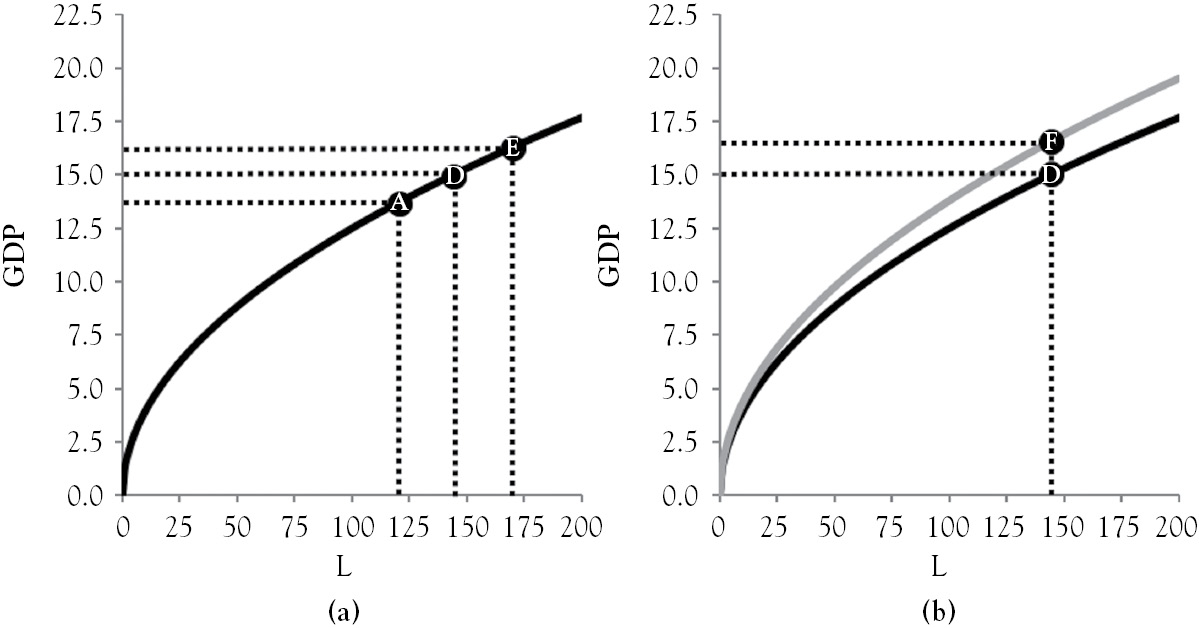
Figure 4.1 The short-run production function
The short-run production function bends because firms’ production lines get increasingly crowded as more and more labor is added. This principle is called the law of diminishing marginal productivity. Production lines get crowded as more labor is hired because physical capital, technology and entrepreneurial talent, and land and natural resources are constant in the short run. If 121 million laborers are in the domestic economy, the economy is at point A, and real GDP equals 13.75 trillion dollars. If 23 million laborers are added, the economy moves to point D as real GDP increases by 1.25 trillion dollars. Adding an additional 25 million laborers pushes the economy to point E, which increases real GDP by another 1.25 trillion dollars. The ratio of the increase in GDP and the corresponding increase in labor is the marginal product of labor, which is $54,348 per worker from A to D and $50,000 per worker from D to E. The marginal product of labor diminishes for any set of three consecutive points plotted on the production function.
If the labor force is initially assumed to be 144 million workers, the economy is at point D in Figure 4.1a, and unemployment would be 0 percent because the number of laborers equals the size of the labor force. This is unrealistic because frictional and structural unemployment are natural. Frictional unemployment arises for voluntary reasons like job dissatisfaction, family moves, or better employment prospects elsewhere. It is not surplus labor, and can be viewed as beneficial because the economy is healthier when workers are taking the time to find jobs best suited for their skills. Structural unemployment is a persistent surplus of labor. It can be caused by a binding minimum wage in low-skilled labor markets; other government interventions like unemployment insurance (UI) compensation, Supplemental Nutritional Assistance Program (SNAP), Medicaid, and other public-assistance programs; employees organized in labor unions; and firms offering efficiency wages to limit employee shirking. It can also be caused by automation that generates an endless cycle of job creation and job destruction. Some structural unemployment is viewed as beneficial because wage offers exceeding the market wage increase productivity and job satisfaction.
To reconcile the conundrum above, the number of laborers is defined to be the employment level (E ) plus the level of natural unemployment. If the natural rate of unemployment is 6.25 percent, 9 million of the 144 million workers are frictionally or structurally unemployed, and the initial short-run production function becomes
This transformation is valid because, again, some unemployment is healthy for the economy. If unemployment equals its natural rate, 135 million workers are employed. Substituting this into the function above gives real GDP equal to 15 trillion dollars. Thus, the transformation allows real GDP and potential output to be equal with nonzero unemployment. In this situation, cyclical unemployment is 0 percent, the quantity of labor supplied (or size of the labor force) equals the quantity of labor demanded (or the employment level) plus the level of natural unemployment, and there is no pressure on wages and prices of other inputs to change.
As mentioned previously, the size of the labor force is considered a long-run variable, even though it can change in the short run. Such changes are triggered by shocks. A temporary extension of UI compensation to 99 weeks can knock the labor force participation rate off its long-run trend for a year. A shift in a demographic trend, on the other hand, can put the labor force participation rate on a different long-run trajectory. For example, the aging of the baby-boomer generation means that an increasing number of workers born between 1946 and 1964 are leaving the labor force as more and more retire.2 Figure 2.6 shows this occurring just after the labor force participation rate peaked in 2000. Over time, such changes tend to slow potential output’s growth rate.
Simulated potential output results when the size of the labor force (Lf) is substituted for L in the economy’s production function:
Substituting the assumed initial values of technology and entrepreneurial talent (1.25 percent), physical capital (0.4 trillion dollars), land and natural resources (2.5 trillion dollars), and the labor force (144 million workers) yields potential output in trillions of dollars:
or
LRAS is a vertical line when graphed with AD, and its location in this graph is determined by the value of potential output. This is so because, in the numerical example above, potential output is 15 trillion dollars whether the PL is 1, 100, 1,000, or any other positive value, and LRAS represents the value of what real GDP should be if real long-run production factors (Z, R, K, and Lf) are fully employed. Initial LRAS and initial AD are graphed together in Figure 4.2 passing through point O.
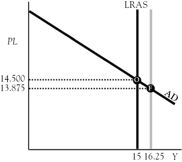
Figure 4.2 AD and LRAS
LRAS shifts to the right if physical capital, technology and entrepreneurial talent, land and natural resources, or the size of the labor force increases. For example, suppose a major technological advancement shifts the economy’s PPF from D to E in Figure 1.7 and rotates the short-run production function counterclockwise from D to F in Figure 4.1b. According to Figure 4.1b, potential output increases to 16.25 trillion dollars. This increase is modeled in Figure 4.2 by LRAS shifting to the gray line. The slide down AD from O to F in this figure suggests that advances in technology, greater investment in physical capital, discoveries of natural resources, or a growing labor force are deflationary.
Short-Run Aggregate Supply
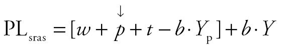
Although LRAS is independent of the PL, SRAS shows the relationship between real GDP supplied and the PL, holding all other influences on production plans constant. SRAS is shifted by several exogenous variables, including the long-run production factors and short-run factors like the nominal wage rate (w), the nominal prices of other production inputs (p), and supply-side taxes (t) (Bade and Parkin 2009). With SRAS’s slope generically defined as b, simulated SRAS is given by
PLsras = [w + p + t – b·Yp] + b·Y
Simulated SRAS can be graphed and analyzed after the slope and short-run production factors are assigned assumed initial values. Suppose the nominal wage rate, the nominal price of other production factors, the supply-side tax rate, and slope b are equal to 7 dollars per hour, 3 dollars per hour, 9 percent, and 1, respectively. Substituting these values and the initial value of potential output, 15 trillion dollars, gives initial SRAS:
PLsras = [7 + 3 + 9 – 1 × 15] – 1·Y
or
PLsras = 4 + Y
Initial SRAS is graphed in Figure 4.3 with AD and LRAS.
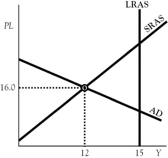
Figure 4.3 AD, SRAS, and LRAS
The intersection of SRAS and AD determines the short-run equilibrium. The first step to finding this involves setting SRAS equal to AD:
4 + Y = 22 – 0.5·Y
Solving this for Y gives an equilibrium real GDP equal to 12 trillion dollars. Substituting this value into either AD or SRAS gives an equilibrium PL of 16 thousand dollars. Thus, the economy is in equilibrium at point O in Figure 4.3. Since real GDP is less than its potential of 15 trillion dollars, unemployment is higher than its natural rate and the economy is said to be in a recessionary gap. If point O had been to the right of LRAS, the economy would have been in an inflationary gap, real GDP would have exceeded its potential, and unemployment would have been below its natural rate. Although output gaps occur in the short run, they do not in the long run. This is so because aggregate factor markets clear in the long run.
A change in a short-run production factor shifts SRAS but not LRAS. For example, suppose government temporarily reduces supply-side taxes from 9 to 7 percentage points. The change is highlighted by the bold number in simulated SRAS:
PL′sras = [7 + 3 + 7 – 1 × 15] – 1·Y
or
PL′sras = 2 + Y
Final SRAS is graphed with initial SRAS and LRAS in Figure 4.4a. The temporary cut in the supply-side tax rate temporarily reduces firms’ marginal costs, shifting SRAS temporarily down to the gray line. If the PL is held constant at 18.5 thousand dollars, real GDP supplied will rise from 15 trillion dollars (point O) to 17 trillion dollars (point F). Because w and p, like t, are added in SRAS’s intercept, a decline in the nominal wage rate or the nominal prices of other production inputs has a similar effect on SRAS as a temporary cut in the supplied-side tax rate.
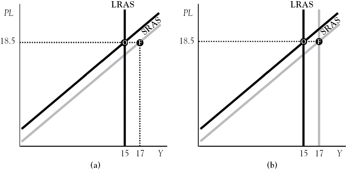
Figure 4.4 Change in a short-run factor versus a change in a long-run factor
Unlike short-run factors, an increase in a long-run factor shifts LRAS and SRAS to the right by the same amounts. Consider a change in immigration policy that boosts the labor force to 184.96 million workers. The change is highlighted by the bold number in simulated LRAS:
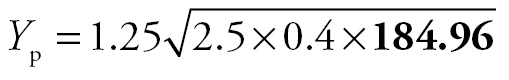
or
With the supply-side tax rate is reset to its assumed initial value of 9 percent, the value of SRAS’s intercept falls when potential output increases, which is highlighted by the bold number below:
PLsras = [7 + 3 + 9 – 1 × 17 ] – 1·Y
or
PL′sras = 2 + Y
Initial SRAS and LRAS are graphed with final SRAS and LRAS in Figure 4.4b, with the initial lines intersecting at O and the final lines intersecting at F. The shift in SRAS is permanent unless immigrant workers are deported at a future date. Like an increase in the size of the labor force, increases in land and natural resources, technology and entrepreneurial talent, or physical capital shift SRAS to the right by the same amount as LRAS shifts by.
The Aggregate Market Model
The aggregate market model is comprised of AD, SRAS, and LRAS, and is graphed in Figure 4.3. It is widely taught in macroeconomic principles courses because it accommodates Keynesians, who focus on the demand side and are concerned with short-run fluctuations, and classical economists, who emphasize the supply side and are concerned with the long-run health of the economy. A more appropriate name for this model is the aggregate product market because GDP is the value of final goods and services produced domestically, and aggregate financial and aggregate resource markets are at work in the background. The aggregate financial market provides the money that buyers use to purchase real GDP, while the aggregate resource market provides the inputs to produce real GDP.
The aggregate market model is useful in understanding how the economy adjusts to short-run fluctuations in real GDP or a deliberate change in fiscal policy. At point O in Figure 4.5a, the aggregate market is in a short-run equilibrium called a recessionary gap. In the absence of SNAP, Medicaid, UI compensation, other government safety nets, and a minimum wage rate, there is much pressure on wages to fall because unemployment is high at point O. In the movie Cinderella Man, James J. Braddock’s (played by Russell Crowe) reservation wage fell substantially when he had to beg for work on the docks after losing his boxing license and using up his family’s savings. With workers bidding down the wage rate, the arrow above w in the equation below illustrates how SRAS self-adjusts, increasing from point O to point B.
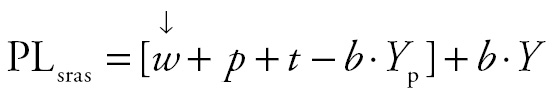
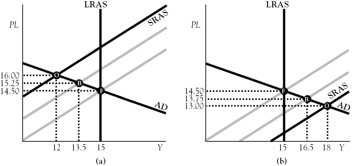
Figure 4.5 SRAS self-adjustment
At point B, the economy remains in a recessionary gap due to slackness in other resource markets. This pushes the price of other production inputs down. The arrow above p in the following equation illustrates how SRAS self-adjusts to shift to point F.
At point F, the output gap is eliminated without government intervention. Allowing SRAS to self-adjust is laissez faire economic policy. The process, however, decreases the PL from 16 to 14.5 thousand dollars, which is why recessionary gaps are also called deflationary gaps. If Medicaid, UI compensation, SNAP, and the minimum wage raise workers’ reservation wages, the gap will close slowly. This is why low-skill wages are said to be “sticky” in the short run.
At point O in Figure 4.5b, the aggregate market is in a short-run equilibrium called an inflationary gap. The name is appropriate because there is upward pressure on prices when unemployment is too low due to real GDP exceeding its potential. When the economy is beyond its PPF, as it is here, resources are overemployed. The tightness in the resource markets causes firms to bid up wages as they try to hire more labor to keep up with rising product demand. The arrow above w in the equation below illustrates how SRAS self-adjusts to point B.
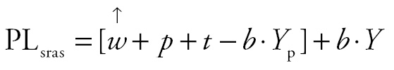
The economy is still in an inflationary gap at point B. This pushes the prices of other production inputs up. The arrow above p in the equation below illustrates how SRAS self-adjusts to point F.
Laissez faire policy allows self-adjusting SRAS to close the inflationary gap, which returns unemployment to its natural rate and raises the PL from 13 thousand to 14.5 thousand dollars.
Fiscal Policy Multipliers Revisited
High unemployment in a recessionary gap and rising prices in an inflationary gap can inflict economic pain. Since upset voters are more likely to vote than satisfied voters (Harpuder 2003), politicians are compelled to act when the economy is in an output gap. These actions are called fiscal policy. In Figure 3.4b, the 0.5-trillion-dollar increase in government expenditure and the subsequent 0.667-trillion-dollar tax cut stimulate AE. This raised real GDP back to 15 trillion dollars, the value that had prevailed prior to the decline in expected future income. This effect, however, rests on the assumption that the PL is constant in the AE model.
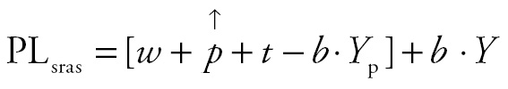
In this chapter, the PL is flexible in the short run due to SRAS’s slope being positive. At point O in Figure 4.6a, the PL is 16 thousand dollars and real GDP is 12 trillion dollars. If government expenditure is raised by 0.5 trillion dollars, AD shifts to point B. The arrow above G in the equation below shows how raising government expenditure affects AD.

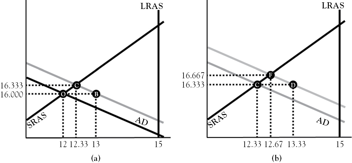
Figure 4.6 Fiscal policy in the aggregate market model
At the moment, the increase in government expenditure is injected into the economy, the PL remains at 16 thousand dollars, and real GDP demanded (at point B) exceeds real GDP supplied (at point O). The resulting 1-trillion-dollar excess in real GDP pushes the PL up to 16.333 thousand dollars at point C. So instead of real GDP rising from 12 trillion to 13 trillion dollars, as seen in Chapter 3, it rises to just 12.33 trillion dollars (at point C). Dividing the rise in real GDP (from O to C) by the increase in government spending gives a multiplier of just 0.667. It implies that real GDP rises by only 67 cents for each additional dollar in government expenditure.
Figure 4.6b shows how a 0.667-trillion-dollar tax cut affects the economy after government expenditures are raised by 0.5 trillion dollars. The arrow above T in the flowing equation shows how tax cuts affect AD.

At the moment, the tax cut is injected into the aggregate market depicted in Figure 4.6b, the PL remains at 16.333 thousand dollars, and real GDP demanded (at point D) exceeds real GDP supplied (at point C). The resulting 1-trillion-dollar excess in real GDP pushes the PL up to 16.667 thousand dollars at point F. As such, real GDP rises from 12.33 trillion to 12.67 trillion dollars. Dividing the rise in real GDP (from C to F) by the size of the tax cut gives a multiplier of just −0.5. It implies that each $1 cut in taxes raises real GDP by only $0.5. If the mpc had equaled 1 instead, the tax cut multiplier would have been equal to −0.667.
The analysis above implies that fiscal policy is not as effective as it appears to be in the AE model. The multipliers above are less than 1 because the absolute value of AD’s slope was assumed to be less than that of SRAS. If the absolute value of AD’s slope had been larger than that of SRAS, the aggregate market multipliers would be larger than 1 but less than their counterparts in the AE model. If SRAS’s slope is equal to zero, the aggregate market multipliers are identical to their counterparts in the AE model. Thus, fiscal policy is increasingly inflationary and ineffective (at closing output gaps) as the slope of SRAS increases. Despite this, fiscal stimulus is sold as a means to close a recessionary gap. This is perhaps due to the resulting budget deficit being financed with bonds that mature after the politicians who enacted the policy have retired.
The Business Cycle
The business cycle refers to the irregular fluctuations in real GDP around its long-run trend, which are plotted in Figure 2.7a. The figure shows real GDP below its long-run trend for the period preceding point E and above it between points E and F. From the Great Recession onward, real GDP has been trending in a deep rut that is parallel to potential output.
The business cycle has two phases, expansion and contraction. An expansion is a period of increasing real GDP, while a contraction is a period of declining real GDP. Since expansions are the norm and contractions are the exception, the long-run average growth rate of real GDP is positive. The transition from expansion to contraction is called the peak, and the transition from contraction to expansion is called the trough. The early portion of an expansion is called the recovery. Although rapid and deep contractions are historically followed by robust recoveries, the Great Recession of 2007 to 2009 was followed by a historically weak recovery.
Because GDP’s long-run trend represents its potential output through time, the economy is at full employment when real GDP crosses over it, as it does at points E and F in Figure 2.7a. Inflationary pressures build as real GDP climbs further and further above its long-run trend, which is the case for periods between points E and F. The aggregate market model equilibrates in inflationary gaps during such periods. Conversely, deflationary pressures build as real GDP dips further and further below its long-run trend. This was the case during the 1991 recession, but deflationary pressures subsided during the periods between the recession’s end and point E. Over this period, the aggregate market model equilibrated in recessionary gaps.
Real GDP’s bumpy ride along its long-run trend is due to AS and AD shocks.3 Supply-side shocks include changes in nominal wages or prices of other inputs to production, technology, government policies promoting or inhibiting entrepreneurialism, subsidies and taxation, regulations that drive up production costs, natural disasters that destroy physical capital used to mine resources or convert raw materials into product, and immigration policies that allow workers of various skill levels to enter domestic labor markets. Demand-side shocks include changes in consumer wealth or expected future income, government purchases, exports, interest rates, investment expenditure, and taxes. Both types of shocks can produce positive or negative effects.
Figure 4.7 shows the effect of a negative shock on the economy that is at full employment. In Chapter 3, the decline in expected future income, from 12 trillion to 11 trillion dollars, triggered a 2-trillion dollar decline in real GDP. Figure 3.4b portrays this as an instantaneous change, but Figure 4.7 shows the economy eventually converging to point F. The speed of this convergence depends on the slope of the AE line. The assumed initial 1-trillion-dollar drop in expected future income shifts AE from points O to I1. The decline in AE causes real GDP to fall by the same amount. This is modeled in Figure 4.7a as the horizontal move from point I1 to the 45-degree line. Because AE’s slope implies that each $1 decline in income reduces planned expenditure by $0.5, AE falls in a second iteration by 0.5 trillion dollars. With the economy at point I2, this process repeats itself in progressively smaller steps until the economy converges to point F. Figure 4.7b graphs the incremental changes in GDP over time, showing the business cycle in a trough in period 4.
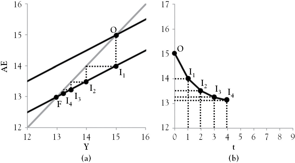
Figure 4.7 The trough of the business cycle
Figure 4.8a shows the effect of a positive shock on the economy that is in a trough in period 4. Although real GDP and AE converge at point F in Figure 4.7, Figure 4.8 shows the economy bouncing off the bottom before it reaches this point. Suppose that the bounce from point I4 to point I5 is caused by the Fed cutting interest rates, resulting in a drop in the real rate of interest and a jump in investment expenditure. At point I5, the aggregate planned expenditure is 1.5 trillion dollars higher than the real GDP, which increases by an equal amount due to firms raising production after observing unplanned drops in inventories. The 1.5-trillion-dollar increase in real GDP is modeled in the figure as a horizontal move from point I5 to the 45-degree line. Since AE’s slope implies each $1 rise in income raises planned expenditure by $0.5, AE rises by an additional 0.75 trillion dollars, which is half of the initial 1.5-trillion-dollar increase in investment expenditure. With the economy at point I6, the process repeats itself in progressively smaller steps until the economy converges to point F′. Figure 4.8b shows the business cycle in a robust recovery from period 4 to 5. The subsequent expansion begins to fade as the economy nears a peak in period 8.
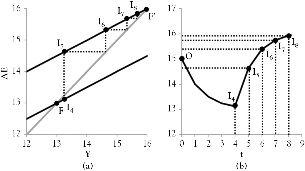
Figure 4.8 The expansion of the business cycle
1 A discouraged worker has given up looking for work because he or she has had no success in finding a job.
2 The U.S. Census Bureau considers a baby boomer to be a person who was born between 1946 and 1964.
3 Samuelson’s (1939) multiplier-accelerator model, which assumes that consumption depends on last year’s income and investment is proportional to the change in consumption, produces a cyclical response to a surge in expenditure.