CHAPTER 5

Current Assets

Chapters 5 through 10 can be thought of as a walk down the Balance Sheet. They will delve into the terms and techniques presented on the Balance Sheet and Income Statement.

Assets, as noted in Chapter 3, are resources that a firm owns or controls. Current assets are those the firm will turn into cash or use within 1 year (i.e., get paid by customers, sell inventory, expire prepaid insurance, and so on). Let us start with the first-listed asset on the Balance Sheet: cash.¹

Cash

Apple, Alphabet (Google), Microsoft, and Exxon are the four largest U.S. (and world) public firms and have lots of cash.² According to their Balance Sheets, the firms’ cash hoards (including cash, cash equivalents, and marketable securities that they could rapidly turn into cash) are as follows:

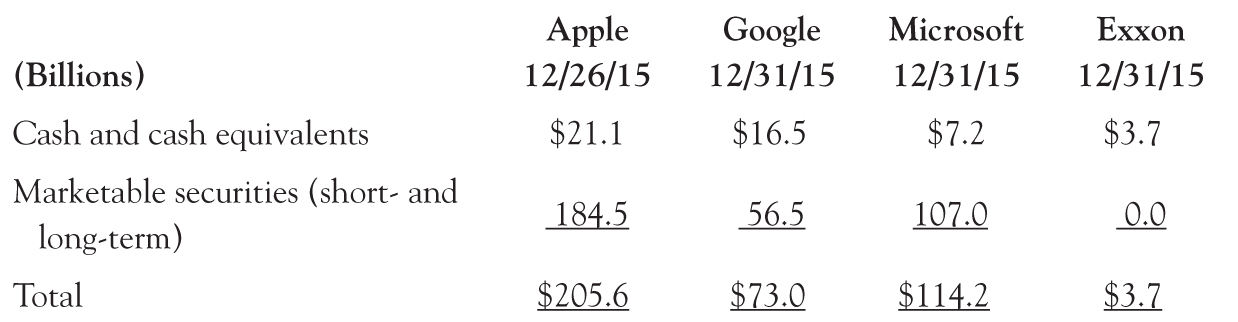
Of all the accounting numbers, cash is the one closest to its true, underlying economic value. But how could cash represent anything but its true underlying economic value? Actually, even cash can have slight differences based on how it is estimated. If all the cash is in one currency (e.g., U.S. dollars), then there is no estimation required and there should be only one number for cash. However, if a firm holds different currencies (as all the firms above do), then the question is how to value the foreign currency. Normally this is done using the year-end exchange rate, but there may be more than 1 year-end exchange rate. There is the bid (the price or rate someone is willing to pay for the currency), the ask (the price or rate at which someone is willing to sell the currency), and the close (the price or rate of the actual final trade). Which exchange (market) should be used? (There are different currency exchanges.) Should the bank commission be included? What about currencies that do not have large active markets? Even for cash, which at first seems to be an easy valuation situation, there may be some assumptions and estimates required. However, differences in the final number should not be very large. Also, there are no alternative accounting choices like those we saw in Chapter 2 for inventory (i.e., first-in first-out [FIFO] and last-in first-out [LIFO]). Cash is a number that is normally as trustworthy as an accounting number can be.

Cash seems pretty straightforward: It is actual currency that the firm holds in one or several bank accounts, and at worst you will have to convert cash held in foreign currencies into the currency in which you are reporting your financial statements.

But what is a cash equivalent? It is a marketable security that the firm could almost instantly convert to cash and something that is expected to become cash in a very short period of time. One common example is a U.S. government debt, money market accounts, and commercial paper that matures within a few months of a firm’s year-end. However, different firms have slightly different definitions for what they include as cash equivalents (again, the Notes to the Financial Statements must be read). Most firms only include items that automatically become cash (i.e., bonds³), excluding even highly traded equities.

For example, Apple’s definition of cash equivalents is:

“All highly liquid investments with maturities of three months or less at the date of purchase are classified as cash equivalents.”⁴

Google has a similar definition:

“We classify all highly liquid investments with stated maturities of three months or less from date of purchase as cash equivalents and all highly liquid investments with stated maturities of greater than three months as marketable securities.”⁵

Note that both firms indicate the securities must mature, which means they are bonds, and the maturity must be 3 months from the date of purchase, which means it is at most 3 months after year-end.⁶

Marketable Securities

If there is an active market where securities (i.e., debt or equity) are actively traded, the securities are considered “marketable.” Shares of Apple Inc. are clearly marketable securities, as would be the debt of the U.S. government (U.S. government debt is the most highly traded of all securities). Interestingly, a firm’s intention often matters in deciding whether an account is considered current or long-term. For example, when Microsoft invested $150 million in Apple Inc. back in August 1997, the investment was meant to last more than a year.⁷ So despite the fact that Microsoft could have sold the Apple shares for cash at any time, the investment was listed as long-term. Intentions matter, and intentions can change. Any time Microsoft decides that it might sell the Apple shares within the next year, the firm can reclassify them as a current asset. If a firm invests in marketable debt securities and the securities will mature in less than a year, then they must be classified as short-term. However, if the debt securities will not mature for more than a year, then the classification is based on management’s intentions.

How are marketable securities valued? At their cost or market price? This is actually a complicated issue. The short answer is, as so often in accounting, “it depends.” Equity securities that are held as short-term assets must be valued “mark-to-market.” This means they must be valued at their market price on the Balance Sheet date. For debt securities held as short-term assets, management has the choice of mark-to-market valuation or using the cost plus accrued interest (accrued interest is the amount of interest earned from the date the bonds were purchased to the Balance Sheet date if no interest is paid in between, or from the last interest payment to the Balance Sheet date if interest is paid after the bonds are purchased but before the Balance Sheet date).

As will be discussed later, firms are sometimes required to reduce an asset’s value when it falls below cost. However, other than for short-term marketable securities, it is rare for firms to increase an asset’s value above cost. Why is the historical cost of an item a core part of valuing assets in accounting? Because the price of an exchange between two unrelated parties (in other words, how much it cost to purchase the asset) is considered a much more reliable and verifiable number than management’s (or their paid proxy’s) estimate of market value. Marketable securities are an exception because there is a reliable and verifiable outside value.⁸

Accounts Receivable

Firms often allow customers a set period of time from when goods or services are delivered until payment by the customer must be made. Common terms would be n/30 (net 30) or n/60 (net 60), which means the payment is expected within 30 or 60 days, respectively. However, sometimes vendors add an incentive to induce their customers to pay earlier. Terms such as 2/10 n/60 means the customer can take 2 percent off the purchase price if payment is received by day 10, otherwise full payment is expected by day 60.⁹ Most utilities and credit cards give consumers n/30 after that there is an interest charged for late payment.

Any amounts owed to a firm by an individual or by another firm can be called a receivable. The bulk of these are owed by customers, and these are called accounts receivables (A/R). We will focus exclusively on A/R, but note that other types of receivables exist.

A firm recognizes (records) revenue when it delivers goods or provides services, as discussed in Chapter 4.¹⁰ If payment is not made at the same time, an A/R is set up. When the financial statements are prepared, the remaining total unpaid receivables are listed on the Balance Sheet. Additionally, an accounting estimate is required to reflect the fact that not all receivables will be ultimately paid. Sometimes, customers will simply not have the ability to pay (e.g., firms enter financial distress and bankruptcy and either pay nothing or perhaps pay some small amount, often the proverbial 10 cents on the dollar, years later). Sometimes, a percentage of customers (hopefully not many) engage in theft and try to vanish without paying.

It may be 6 months to a year before a firm realizes a specific customer will not pay. In order to match the cost of uncollected sales (called bad debts expense) into the same period as revenues (the sales of the goods and services), an estimate of what will ultimately not be collected is made.

How do accountants make a year-end estimate of what will be ultimately not be collected (called allowance for doubtful accounts [ADA])? There are several different ways. One is to examine each customer and estimate whether the payment will be made. This is very time consuming and is done only for very large or key customers. The more common methods are to use either a percentage of credit sales (total sales are used if the breakdown between cash sales and credit sales is not known) or through a process known as aging of accounts receivable. Both methods of estimating the ADA (i.e., the Balance Sheet amount) and bad debt expense (i.e., the Income Statement amount) include historical firm and industry experience along with expectations of how the overall economy will do (if the economy is heading into a recession, the estimated collections may be reduced, whereas when the economy is coming out of a recession, the estimated collections may be increased).

These two methods, Percentage of Sales and Aging of Accounts Receivable, also illustrate how the choice of accounting method creates a trade-off between the Balance Sheet and the Income Statement. That is, the choice of the accounting method determines whether the firm’s Balance Sheet better reflects (is closer to) economic reality or whether the firm’s Income Statement provides better guidance in predicting future cash flows. The percentage-of-sales method is an Income Statement approach in the sense that it does a better job of matching costs to revenues. The aging method is a Balance Sheet approach in that it provides a better estimate of the amount that will actually be collected.

In other words, the more accounting focuses upon Balance Sheet valuations the greater the potential distortion in the Income Statement. Conversely, the more accounting focuses upon income measurement the greater the potential distortion in the Balance Sheet. This is not just true for bad debts, it is true for numerous measurement issues as will be shown in later chapters.

Percentage of Sales

Let us start with the Percentage of Sales (% Sales) method. How does this method work? At year-end, management estimates the percentage of sales that it expects it will be unable to collect (using the firm’s historical experience combined with industry and economic trends).

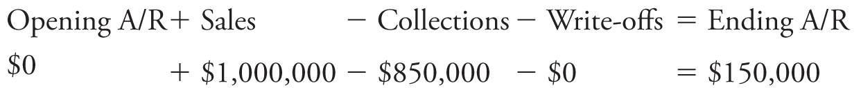
As an example, assume a firm has annual sales of $1 million and that, to keep the example simple, all the sales were on credit. It is the firm’s first year of operations, so the firm does not have any uncollected amounts that carried over from the prior year (i.e., the opening balance of A/R is $0). Of the $1 million in sales on credit this year, the firm has collected $850,000 by year-end. The firm’s customers therefore together owe the remainder of $150,000 ($1 million − $850,000 = $150,000). In other words, the firm has an Accounts Receivable balance of $150,000 (Remember, the amount on the Balance Sheet for A/R is a total of numerous customers). The formula to compute A/R is:

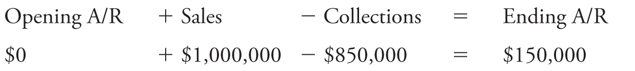
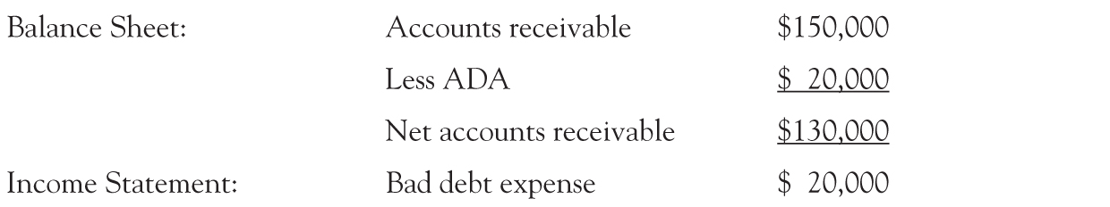
If the firm estimates that 2 percent of sales will never be collected, this translates to an estimate of $20,000 (2 percent of $1 million). The firm would show “net” A/R of $130,000 (the $150,000 less the $20,000 that it expects not to collect). The firm would also reduce profits by $20,000 (matching the cost of the uncollected amounts, or bad debts, to the revenues), thereby reducing the year-end Retained Earnings account.

Note that the firm is setting up an estimated amount for the total amount it expects not to collect. It does not adjust the actual individual customer accounts until it knows which specific customer(s) will not pay, which means it does not change A/R itself. Why not? It is because the amount on the Balance Sheet for A/R is the total of numerous customer accounts that owe money to the firm. The firm does not yet know which customer’s account to reduce. Thus, a new account is created called ADA (allowance for doubtful accounts) that reflects the estimate of what will not be collected. This is a contra or negative asset account (it is increased with a credit and reduced with a debit) in that it is attached to an asset account (e.g., A/R) and reduces it (as opposed to reducing the individual accounts that make up A/R). Thus, there are many individual customer accounts totaling $150,000 (with a debit balance) and there is the new ADA showing a year-end balance of $20,000 (with a credit balance). The Balance Sheet can show both but usually just shows the net of $130,000.

Remember: The ADA is a Balance Sheet number reflecting the amount a firm expects not to collect. The bad debt expense is an Income Statement number reflecting the amount of non-payments matched to this year’s revenues.

In the first year, there is no trade-off between the Balance Sheet valuation of receivables and the income measurement because bad debt expense and the ADA are the same. This will change once estimates do not match actuals in future years.

Assume that in its second year of operations, the firm actually collects $135,000 of the first year’s year-end A/R. This means the firm made a mistake in its first year financial statements by overestimating the ADA and the bad debts expense. The first year’s Income Statement was $5,000 lower than it would have been had management estimated correctly (at $15,000 instead of $20,000). Reported total assets and retained earnings were also $5,000 lower than they would have been. However, the Balance Sheet and Income Statement of the first year are not corrected for this type of mistake. At the time the statements were prepared, the numbers were based on the best estimate available. The only time prior year’s statements are changed is when there was a major numerical mistake, a case of fraud, or when the government mandates a change in an accounting choice with a retroactive change in prior year’s numbers. The fact that an estimate later proves to be wrong does not by itself lead to changes in prior year’s financial statements.

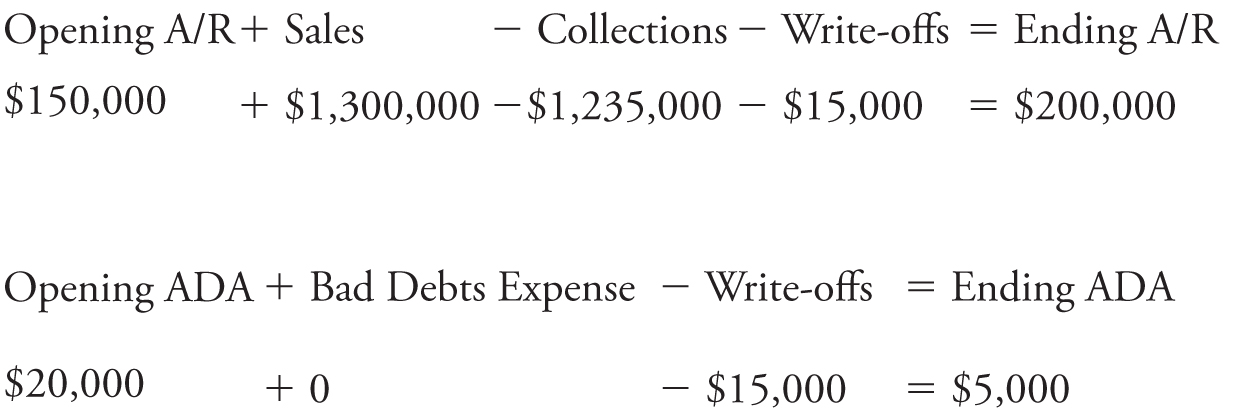
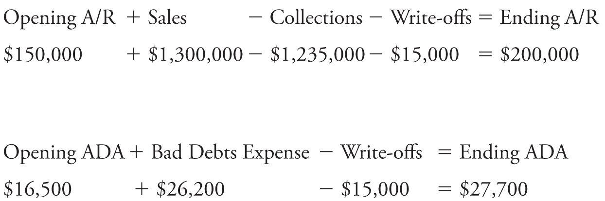
Now assume that the same firm has sales of $1.3 million in the second year, of which it collects $1.1 million. Remember, we said above that in the second year, the firm also collects $135,000 of the A/R from the first year. How much is the firm owed at year-end? The answer should be $200,000 ($1.3 million less $1.1 million), but until adjustments are made the A/R balance will be $215,000. This is because the math of the A/R accounts, prior to an adjustment to the ADA, is as follows:

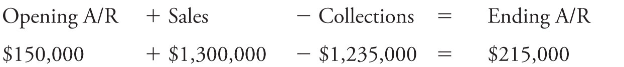
The amount owed at the start of the second year is same as the first year’s ending balance which is the total A/R of $150,000. Sales during the year were $1.3 million. The firm collected $1,235,000 ($135,000 of the amount owed from the prior year plus $1.1 million of this year’s sales).

At some point (the firm can do it at any time of its choosing), the firm will recognize the $15,000 that it will definitely not collect and “write off” the specific customer accounts (remember, the A/R at the end of the first year was $150,000 and in the second year only $135,000 of that was collected, leaving an actual uncollected amount of $15,000). The write-off is done by reducing the appropriate individual customer accounts and by reducing the ADA. For example, imagine Clown Costume Inc. (CCI), which owed $15,000 filed for bankruptcy and is expected to be unable to make any payments. The account of CCI is reduced (credited) by $15,000 (with a note it is for lack of payment) and the ADA account is reduced (debited) by $15,000.

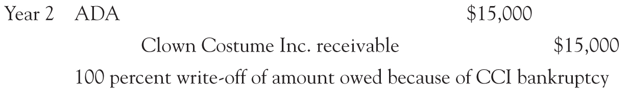
Thus, we restate the A/R equation as follows:

Accounts receivable reflects the amount owed after adjusting for those specific customers which the firm has recognized will not pay.

An aside: In the individual customer accounts, the firm will keep track of the write-off. The account will be tagged to indicate that it has been reduced to zero not because the customer paid but because it was written off as uncollectible. If the customer ever returns and wants to purchase merchandise, the firm may refuse because of the prior nonpayment or may ask the customer to first repay what had been owned plus a “finance fee.”

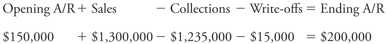
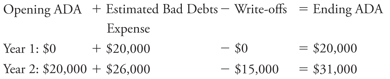
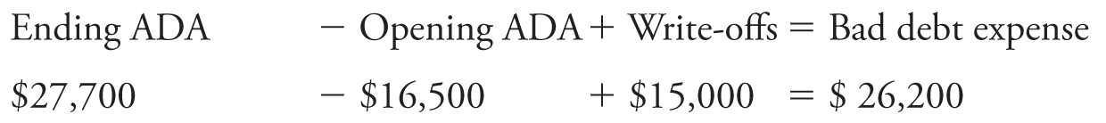
The ADA, as noted previously, is a contra or negative account on the Balance Sheet. It reduces the net A/R shown on the Balance Sheet. The formula for the ADA is as follows:

Opening ADA + Bad Debts Expense − Write-offs = Ending ADA

Note, the write-off lowers both the A/R and the ADA, so it has no effect on the net A/R.

For example, prior to the write-off (and an adjustment for this year’s bad debt expense), the A/R was $215,000 and the ADA was $20,000 for a net of $195,000.

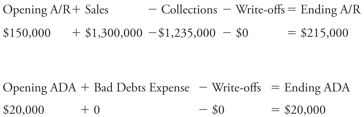
After the $15,000 write-off (and still before an adjustment for this year’s bad debt expense), the A/R is $200,000 and the ADA is $5,000 for a net of $195,000.

Under the Percentage of Sales method, the Income Statement amount for bad debts expense is estimated as a set percentage of credit sales. In the first year, the bad debt expense and the ADA are the same (assuming no write-offs in the first year). In future years, the bad debt expense and year-end ADA are unlikely to be the same because prior year’s mistakes remain in the ADA.

Remember, the ADA is a Balance Sheet account and, like all Balance Sheet numbers, it is cumulative, showing the value as at an instant in time. However, because of how it is computed it accumulates mistakes over time. The Percentage of Sales method estimates each year’s bad debt expense. To the extent the estimate is wrong, the Income Statement and ADA are wrong. However, unlike the Income Statement number, the ADA is not reset to zero each year. Under the Percentage of Sales method (again, where bad debts expense is being calculated), the ADA is increased by bad debts expense and reduced by write-offs, which means past year’s errors will cumulate over time when using this method.

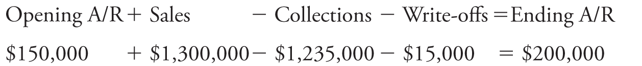
Assume that at the end of year 2, the firm still estimates that 2 percent of sales will not be collected; this would mean that the estimate for year 2’s bad debts expense is $26,000 (2% × $1.3 million). The equation for ADA for years 1 and 2 is as follows:

The estimate for bad debts expense does not affect A/R, which remains at $200,000:

This means that the year 2 ending net A/R on the Balance Sheet is $169,000 (ending A/R for year 2 of $200,000 minus the ending ADA for year 2 of $31,000).

As can be seen previously, the ending ADA is $31,000 (or $5,000 more than the current year’s bad debt expense of $26,000). The $5,000 mistake from the overestimation of bad debt expense in year 1 is left on the Balance Sheet, which increases the ADA from $26,000 to $31,000 and reduces the net A/R from $174,000 to $169,000.

Why not adjust the Balance Sheet to take into account the prior year’s overestimation? It is because, as noted, the Percentage of Sales method is an Income Statement approach. This means that this method is trying to match revenues and costs (bad debt expense is a cost). The best estimate of this year’s bad debts is $26,000. This is the best number to match against this year’s revenue.

In order to adjust the Balance Sheet’s net A/R to the more accurate value of $169,000 requires a $5,000 adjustment to both the Balance Sheet ADA account and the Income Statement bad debts expense. This means, in order to remove the prior year’s overestimation of $5,000 requires this year’s bad debt expense to be lowered from $26,000 to $21,000. However, using an amount of $21,000 for year 2’s bad debt expense does not fulfill the Percentage of Sales method’s goal of matching costs (which is $26,000 in year 2) to that year’s revenues.

The firm made a mistake last year when it estimated bad debts to be $20,000 and ultimately only $15,000 were not collected. The firm has two choices: (1) leave the mistake on the Balance Sheet and properly match this year’s revenues and costs with a bad debt expense of $26,000 or (2) adjust the prior year’s error on this year’s Income Statement by reducing bad debt expense to $21,000 and thereby removing the $5,000 mistake from the Balance Sheet, which would then show the year-end ADA as $26,000 instead of $31,000. The Percentage of Sales method chooses option (1) and leaves the error on the Balance Sheet. Again, the Percentage of Sales method is an Income Statement approach and focuses on matching a year’s cost to that same year’s revenues.

Using the Percentage of Sales method, the mistakes usually average out over time because of overestimating one year and underestimating the next. It is possible for a firm to continually over- or underestimate, but at some point if the ADA account becomes too large it must be reduced by using a lower amount of bad debt expense – in that year the firm will not match costs to revenues as well.¹¹

Aged Accounts Receivable

By contrast, the Aged Accounts Receivable (Aged A/R) method is a Balance Sheet approach that tries to reflect the true economic value of the Balance Sheet item. This means that at the end of each year, the ADA on the Balance Sheet is adjusted so the net A/R is set at what is expected to be collected. Doing so means that bad debts on the Income Statement is adjusted for prior errors and will not match as well as under the Percentage of Sales method.

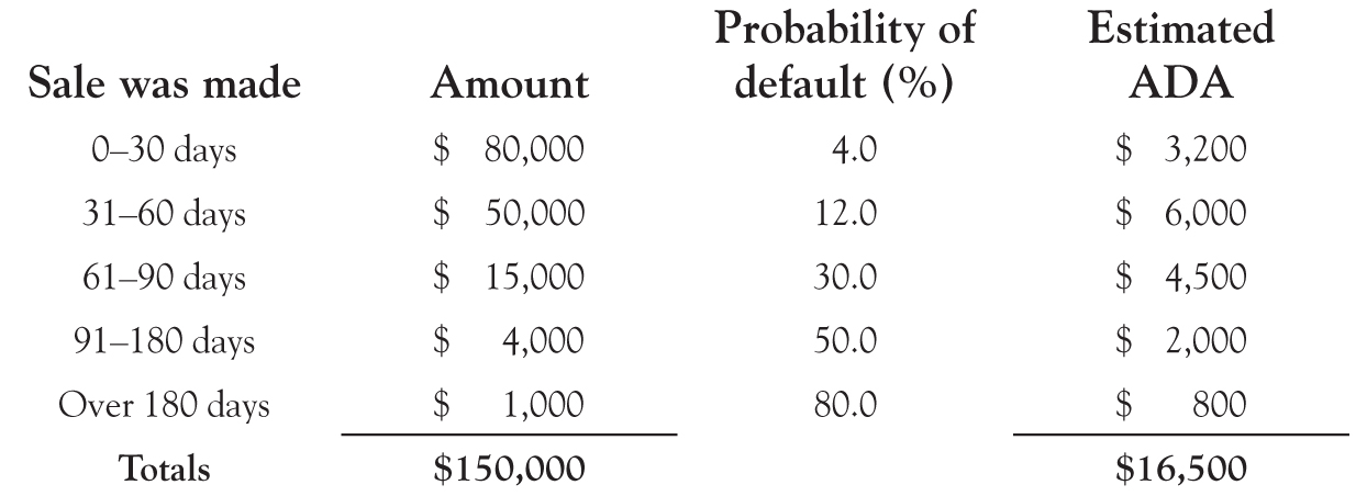
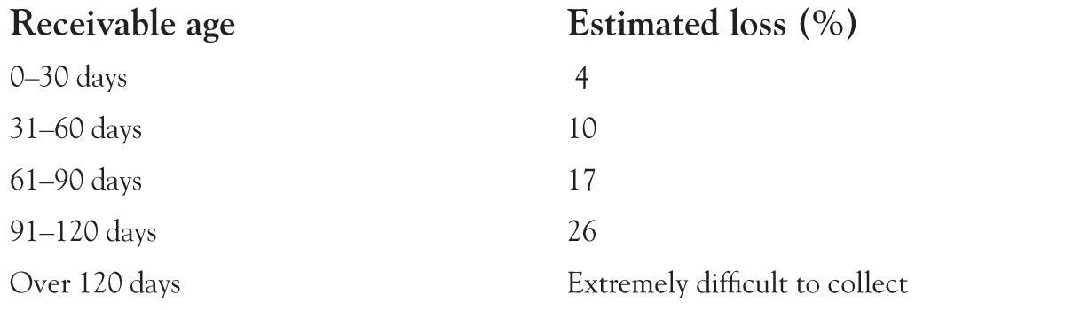
The Aged A/R method computes the ending ADA. This is done by first listing each individual uncollected sale at year-end by age (i.e., by how much time has passed since the sale). As an example, let us again assume that the firm ended its first year with A/R of $150,000. Let us further assume they are aged as follows:

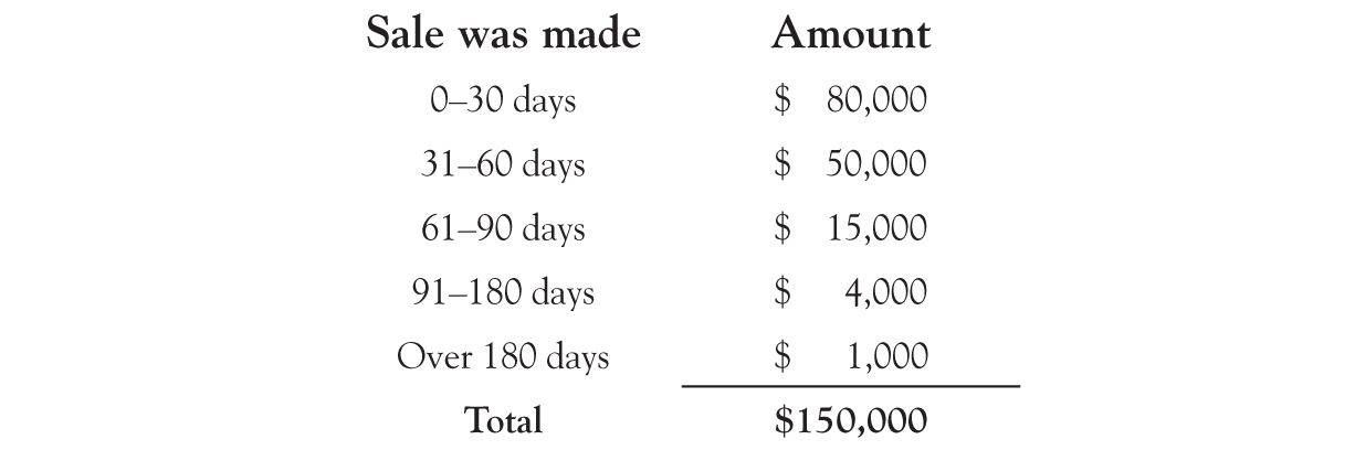
The firm estimates an uncollectible rate for each time period (category). Note that if the firm has given customers 30 days to pay, then the $80,000 sold within the last 30 days is not yet late. The more time has passed since the sale was made without payment, the less likely it is that the firm will ultimately be able to collect payment and the higher the default probability. For example:

There are several items to note at this point. First, the estimates under the two methods (% Sales and Aged A/R) are not likely to produce the same ending net A/R amounts. Second, aging is generally thought to be a more accurate estimate of what will ultimately be collected because it is more specific and takes into account what has been collected to date (while, as noted previously, % Sales does a better job of matching). Finally, and most importantly, the amount being estimated under the Aged A/R method is NOT bad debt expense. Rather, the amount being estimated is the ending ADA amount (remember, the amount being estimated under the % Sales method is the bad debt expense). This means we compute ending ADA and solve for bad debts expense:

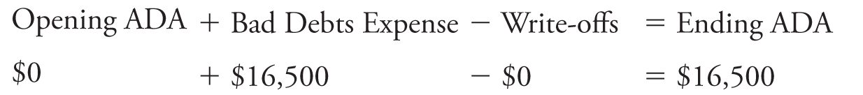
Opening ADA + Bad Debt Expense − Write-offs = Ending ADA

Ending ADA − Opening ADA + Write-offs = Bad Debt Expense

 

Continuing our previous example, in the first year the ADA and bad debt expense are the same amount ($16,500) because in the first year there are no opening ADA balances and no write-offs.

Our first year-end A/R is unchanged as follows:

Thus, the ending net A/R value is $133,500 because the bad debt expense and ADA are now $16,500 (instead of the $20,000 under the % Sales method) because of the different estimation.

For simplicity, we estimate the second year-end ADA with the same percentages for each category as in year 1:

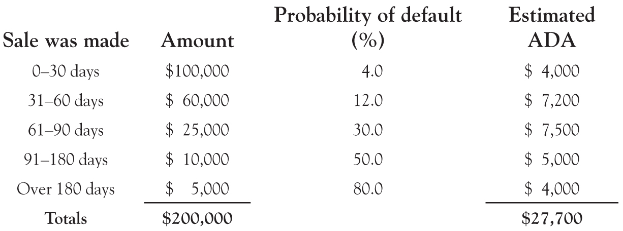
This means that at the end of the second year, the net A/R on the Balance Sheet is $172,300 (the ending A/R of $200,000 minus the estimated ADA of $27,700) and the bad debt expense on the Income Statement is $26,200.

The bad debts expense was estimated by solving the equation as follows:

As noted previously, the different methods result in different estimates. In the % Sales method above, the first year estimate was $20,000, whereas in the Aged A/R method, it was $16,500. The actual amount turned out to be $15,000. This means the first method overestimated bad debts expense by $5,000, whereas the second overestimated bad debts expense by $1,500.

Additionally, the % Sales method leaves prior year’s error in the ADA. By contrast, the Aged A/R method moves the error to the bad debts expense. This can be seen here as the ADA is calculated as $27,700 but the bad debt expense is $26,200. The $1,500 difference is the prior year’s error (using the Aged A/R method). Essentially, since the ADA reflects the year-end estimate of what will be collected, the prior year’s error is included in bad debts expense (in this example lowering it by $1,500). Thus, the Aged A/R method produces a Balance Sheet closer to economic reality in terms of what the firm expects to collect. However, the Aged A/R method does not match costs to revenues as well as the % Sales method does.

Although there are no set guidelines, a U.S. Department of Commerce study provides the following:¹²

 

Inventory

In a retail operation like our T-shirt vendor example in Chapter 2, items are purchased and resold. Purchases of inventory are listed under current assets until they are sold (inventory increases and cash decreases if the firm pays immediately, or inventory increases and accounts payable increases if the firm purchases the inventory on credit). When the items are sold, inventory is reduced and an Income Statement account, which matches the cost of the T-shirts to revenue, called cost of goods sold (COGS) or cost of sales is created. The equation for the account is below, followed by Walmart’s numbers for the year ending January 31, 2016.

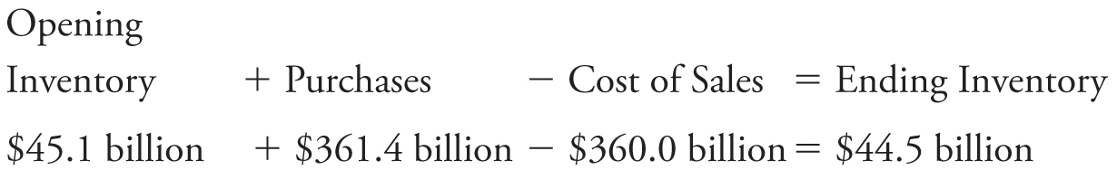
Note that the opening and closing inventory numbers come from the Balance Sheet, whereas the cost of sales number comes from the Income Statement. Purchases is not provided in the financial statements and must be computed as follows:

Purchases = Ending Inventory + Cost of Sales − Opening Inventory

Walmart includes in cost of sales not only what it paid for the merchandise it has sold but also the costs of its distribution and warehouse facilities. Likewise, the ending inventory is not only what Walmart has in its stores but also what it has in its warehouses.

In a manufacturing operation, the accounting process is more complex. First, there are three broad categories of inventory (and within each there may be thousands of individual accounts, one for each item at each location):

       Raw materials (the unchanged inventory that goes into the final products),

       Work-in-process (partially made products), and

       Finished goods (the final products ready to be sold).

The complexity occurs when computing work-in-process. As a product is being made, raw materials are transferred both literally and in the accounts: The raw materials move out of the raw materials account (with a credit) and into work-in-process (with a debit). However, work-in-process is also increased for all the costs of manufacturing. These costs include direct labor, which is the costs of wages and related benefits of all the employees who work directly on the product. The costs also include the cost of operating the plant (e.g., rent, electricity, and maintenance) referred to as overhead. The equation can be written as follows:

Work-in-Process_start + Raw Materials + Direct Labor + Overhead − Cost of Goods Manufactured = Work-in-Process_end

There are a variety of ways to allocate overhead costs to specific products, but often it is done simply as a percentage of direct labor. For example, if the total cost of operating a plant is $1.5 million and the total direct labor in the plant is $1 million, then the relationship of overhead to direct labor is 1.5 ($1.5 million / $1 million). The direct labor is traced to individual products (i.e., with time cards) and the overhead is applied at a rate of $1.50 per $1.00 of direct labor. Imagine the firm has only three products, A, B, and C. Each product is charged for the actual raw materials and direct labor used. Assume A uses $200,000 of raw materials and $600,000 of direct labor, B uses $400,000 of raw materials and $350,000 of direct labor, and C uses $25,000 of raw materials and $50,000 of direct labor. The $1.5 million of overhead is applied based on the direct labor, and the product costs would be as follows:

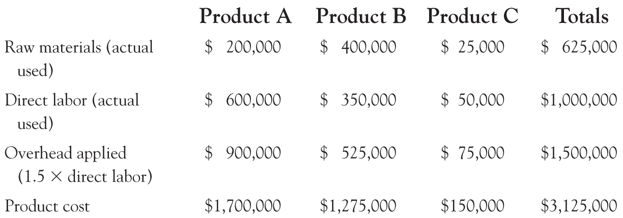
As the product is completed it moves out of work-in-process (with a credit) and into finished goods inventory (with a debit). Then, when it is sold, the process is the same as for a retailer: Finished goods inventory is reduced (with a credit) and COGS is increased (with a debit).

To determine the amount to reduce (credit) the inventory account, the firm must apply a cost or price to the product. Whether the product is manufactured or is purchased in the form it will be sold, prices can vary over time. This takes us to the question of how to cost the inventory as it is sold, a topic already introduced back in Chapter 2. There are four methods generally used. They are as follows:

    •   Specific identification,

    •   FIFO,

    •   Average, and

    •   LIFO

Specific identification is normally restricted to high-value items where the customer selects a specific product. Remember, there will be an inventory category for each type of product (each model, variety, size, fabric, and so on). Clearly a customer will not care which of three identical T-shirts she gets. By contrast, someone purchasing a car is likely to not only want a specific model but also care about color and optional features. Thus, a local car dealer might use specific identification to cost inventory. However, the automobile manufacturer, which sells anywhere from tens of thousands to millions of a particular model, would not use specific identification. Likewise, a single retail jewelry store might use specific identification on some of its very expensive jewelry (e.g., diamond rings selling for over $10,000). The benefit of specific identification is that it matches the cost exactly to the revenue. The disadvantage is that when items are not differentiated, as in the case of the identical T-shirts, management could manipulate profits by choosing which specific (though identical) item is sold, essentially picking the cost that the firm will report. Also, this method may be more expensive to implement as it requires that the firm track exactly which item sold.

FIFO, Average, and LIFO are the three most common methods used. Average is just that, somewhere in the middle. Let us delve into FIFO and LIFO again.

FIFO is a Balance Sheet approach. It reduces the value of inventory on the Balance Sheet, and increases the Income Statement expense (called COGS) when items are sold in the same order as they were purchased. As the name implies, first-in first-out. This also means FIFO values ending inventory using the cost of the last items purchased, which is a value closer to replacement cost. Remember our T-shirt example with three items purchased for $10, $12, and $14. If FIFO is used, when one item is sold its cost is $10 which is the cost of the first inventory item purchased, whereas the remaining T-shirts (i.e., the ending inventory) are together valued at $26 ($12 + $14). The $26 is less than the likely replacement value of $28 (2 × $14), which is what the firm would have to pay to replace the two remaining T-shirts if the cost was the same as the $14 it paid for the last one. However, the FIFO value is closer to replacement cost than the LIFO value as explained below.

LIFO is an Income Statement approach. LIFO costs (reduces inventory value and increases COGS) in the reverse order of that purchased. As the name implies, last-in first-out. This makes the Income Statement expense more representative of the likely future costs and thereby provides a better estimate of future cash flows (assuming the firm maintains a constant or increasing quantity of inventory). In our T-shirt example, using LIFO, when one item is sold its cost is $14 which is that of the last inventory item purchased. The remaining T-Shirts are together valued at $22 ($10 + $12).

The FIFO ending inventory value on the Balance Sheet is closer to replacement value because it includes more current prices. However, the Income Statement using FIFO is not as good an estimate of future profits because it includes older purchase prices. The LIFO ending inventory value on the Balance Sheet is not as close to replacement value because it uses older purchase prices. However, the Income Statement profit gives a better estimate of future profits because it uses more current costs. The trade-off between the two methods, FIFO and LIFO, is the same trade-off as between the Aged A/R method (like FIFO, a Balance Sheet approach) and the % Sales method (like LIFO, an Income Statement approach).

LIFO has one very important caveat: It provides management the possibility to manipulate reported profits by undertaking the economic action of reducing the firm’s physical quantity of year-end inventory. Consider again the T-shirt vendor in Chapter 2. Assume the firm starts the year with three units of inventory that cost $10, $12, and $14 for a total of $36. Regardless of whether the firm purchases any additional units, FIFO will always cost the sale of the first unit of inventory at $10 regardless of when it occurs. However, for LIFO, the cost is $14 if the firm purchases no new inventory during the year. If the firm buys another unit for $15, then under LIFO the cost of the unit sold is $15 because LIFO stipulates that the cost of the unit sold is always the cost of the last unit purchased. Now imagine the firm bought no new inventory during the year. It would cost one unit at $14 (rather than $15, which appears to be the new market price), as shown in the example below. In subsequent years, if no new inventory was purchased, it would cost the next unit at $12 (rather than some amount above $15 if prices keep rising).

As shown below, failing to replace units sold makes no difference for FIFO but can affect LIFO:

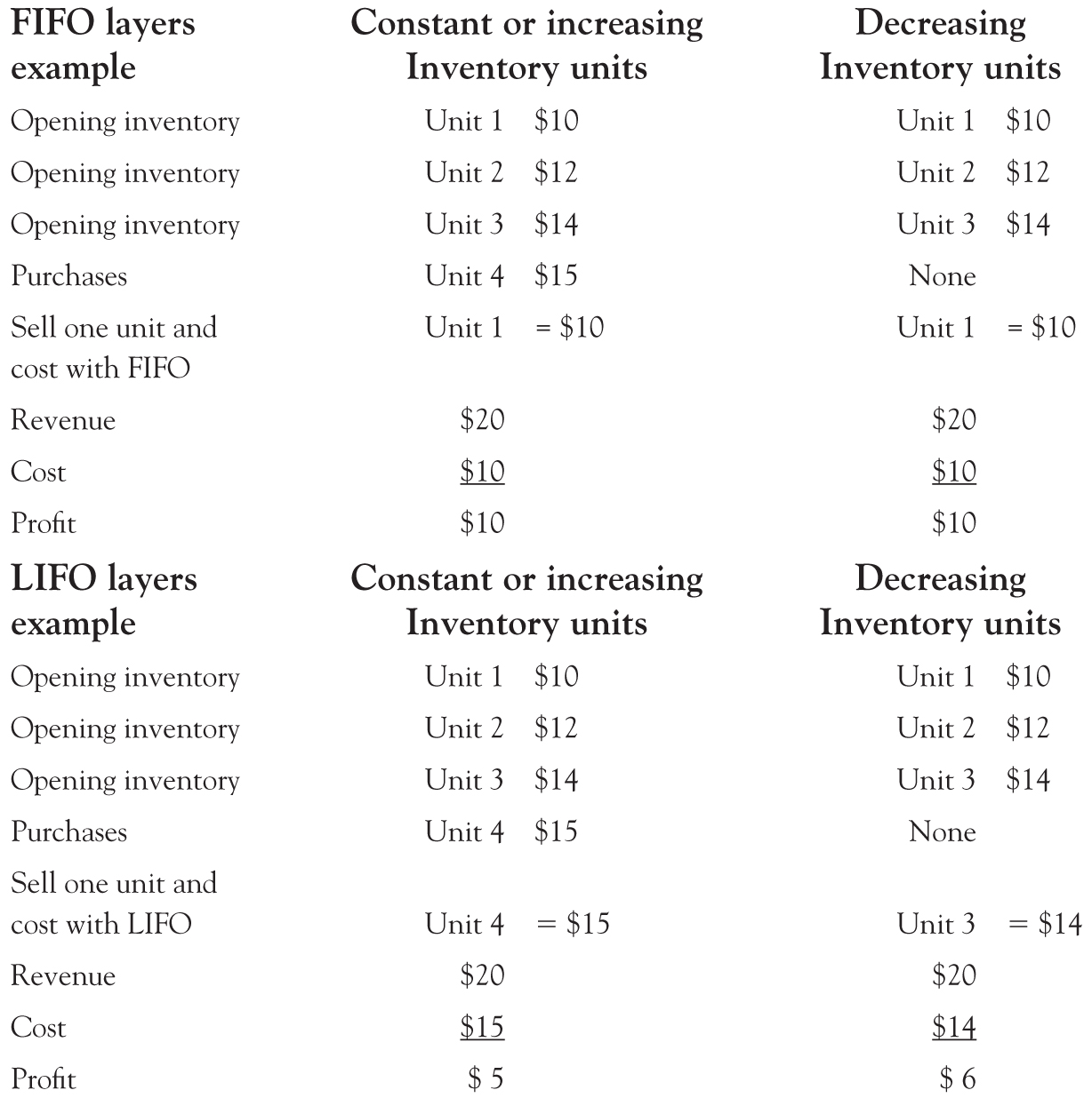
A firm using LIFO which increases its profits by selling inventory and not buying replacements and thereby reducing the quantity of year-end inventory (in this case from three to two units) is said to be “eating into the LIFO layers.” (Note, we normally assume prices are rising, but this is not always true. If prices are falling, LIFO produces a higher profit than FIFO.)

The above also assume inventory costing is done once a year, which used to be true before the advent of computers. Today, many firms use what is known as perpetual costing, which means the costing is done each time a unit is sold. This makes the timing of purchases and sales important. Consider the following scenarios:

    •   Purchase a T-shirt for $10,

    •   Purchase a T-shirt for $12,

    •   Sell a T-shirt for $20, and

    •   Purchase a T-shirt for $14

If inventory costing is done periodically (e.g., once a year), then the LIFO cost of the one unit sold is $14 because that was the cost of the last unit purchased in the year. However, if the costing is done perpetually, the LIFO cost is $12, (and the ending inventory is $24 ($10 + $14), because when the T-shirt was sold the cost of the latest purchased item was $12.

One last inventory point before a couple of interesting stories. Inventory is valued at the lower of cost or market. Cost is determined as above, using FIFO, Average, or LIFO. Market is the selling price (minus certain direct selling costs, like commissions). If the market is less than cost, then the inventory has to be written down to market, and this becomes the new cost (by convention it is not written back up if the market value increases in the future).

The LIFO vs. FIFO Controversy

What method would you, as manager of a firm with rising inventory prices, want to use for your public financial statements, FIFO or LIFO? Probably FIFO. Why? Because if prices are rising, FIFO will show higher profits than LIFO. What method would you prefer to use on your Income Tax returns? LIFO. Why? Because if prices are rising, LIFO will show a lower profit than FIFO and allow you to delay taxes.

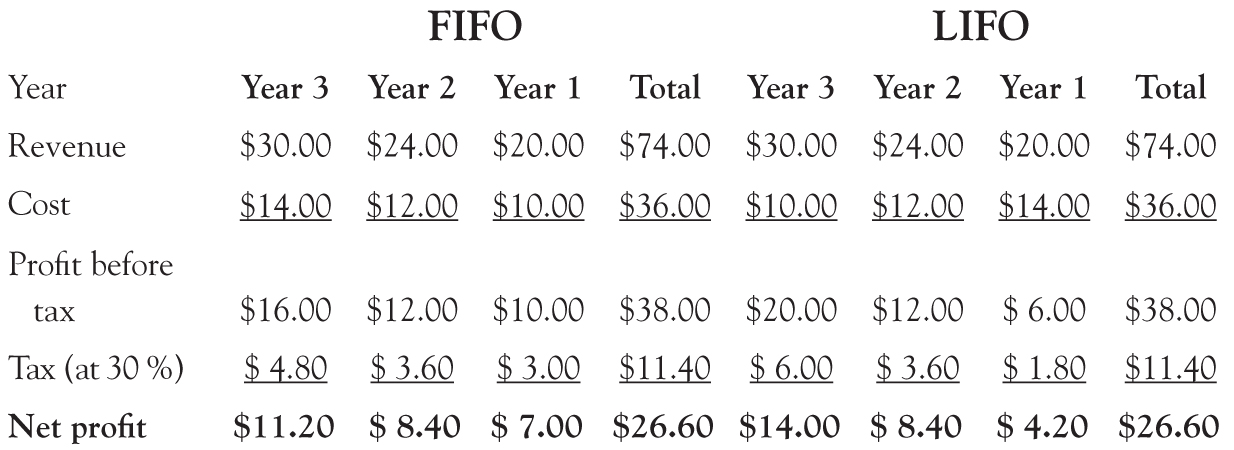
Back to our T-shirt vendor. Imagine you purchase the three units up front for $10, $12, and $14. Then you sell one T-shirt a year for $20, $24, and $30. To show the highest possible profit during the first year, the firm chooses FIFO and then is “locked in” to this accounting choice because changing accounting choices requires an explanation and a transition year with two sets of financial statement numbers. The firm’s profits before taxes over the 3 years are $10 in the first year ($20 − $10), $12 in the second year ($24 − $12), and $16 in the third year ($30 − $14). If taxes are based on these FIFO-induced profits and the tax rate is 30 percent, the firm will owe the government annual taxes of $3, $3.60, and $4.80, respectively.

By contrast, using LIFO will show profits before tax of $6 in the first year ($20 − $14), $12 in the second year ($24 − $12), and $20 in the third year ($30 − $10), with taxes equaling $1.8, $3.6, and $6, respectively. Notice that when we sum total profits before or after tax over the 3 years, FIFO and LIFO result in the same 3-year sums ($38 and $26.60, respectively). This also happens when we calculate total tax over the 3 years ($11.4).

If the firm will end up paying the same aggregate amount in taxes in the long-term, why would it want to pay lower taxes now? Paying the government later is generally preferred, as you can invest the funds you do not give the government or borrow less. Essentially, by using LIFO for tax purposes, you are able to delay a $1.2 payment from Year 1 to Year 3. The amounts become interesting once they are in the millions, let alone the $36.8 billion Exxon has currently delayed paying.¹³ (Chapter 8 provides a detailed discussion on the time value of money.)

This means that firms with rising inventory costs would likely prefer to use FIFO for the public (as it shows higher profits) and LIFO for the government (as it delays paying taxes). Unfortunately, back in 1971, LIFO was not allowed in the U.S. for tax purposes and, since prices were rising, most firms used FIFO in their public reports in order to report higher profits to the public. After a considerable amount of lobbying in 1972, Congress decided to allow firms to use LIFO for tax purposes. However, Congress inserted an important caveat, firms could only use LIFO for tax purposes if they also used LIFO in their public reports.¹⁴

The above means a firm would save money by switching from FIFO to LIFO by deferring tax payments but would have to report lower current accounting profits to the public in order to do so. This is an important point: Economically the firm would have higher cash flows this year by deferring some of its tax payments, but to do so, it would have to lower current reported accounting profits. Remember, as shown in the example above, over the long-term it makes no difference.

Would you, as a manager, make the switch? Do you believe the market will understand what you are doing or punish you for lowering profits? In 1973, eight firms listed on the Compustat database switched from FIFO to LIFO. Their stock price rose, as apparently the market understood and appreciated what they did. The next year 183 firms switched from FIFO to LIFO.¹⁵

At one point, because of this tax effect, a majority of U.S. firms used LIFO. Today the number is much less (one study of 5,000 public firms puts the number at around 8.7 percent).¹⁶ There is also a downside risk to using LIFO in periods of rising prices – liquidating inventory can increase profits but may result in unexpected tax liabilities. Finally, a new problem with LIFO has arisen. Under IFRS, which are used by the European Union and others, LIFO is not allowed.¹⁷

What will the U.S. regulators do in response to IFRS? We shall see. (Your author is betting on the U.S. continuing to allow LIFO for tax purposes even if U.S. financial reporting standards are changed to align with IFRS by prohibiting LIFO or Congress repealing the LIFO conformity rule.)

An Accountant in Dallas (Based on the 1978 TV Show Dallas)

A young man named John Ross sets off to seek his fortune. He finds it in the oil industry and becomes very wealthy. Along the way, he not only cheats his business partner but also steals his partner’s girlfriend, who he marries and with whom he has three sons. The eldest of his sons, named JR (after himself), is pure evil. The youngest, named Robert, is a great guy who is constantly being abused by JR. The middle son is ignored.

When John Ross dies, there was one especially interesting element in his will: John Ross had decided he wanted whichever son was better at managing the business to run his empire (no first-born rights to the kingdom for JR). JR and Robert would each get one division of his business. Then, whichever son earned more in the next 6 months would become chief executive officer (CEO) and control the empire. Of course, measuring who earned more is based on, you guessed it, ACCOUNTING!

JR was given the retail division, comprised of a chain of gas stations selling fuel. Robert was given the exploration division, which searches for new oil. JR would generate profits from the ongoing business of selling oil at retail for more than it cost. Robert had to find oil and then sell it wholesale in 6 months. Let me provide numerical assumptions (something the TV show never discussed).

Assume Robert is given $30 million to explore for oil and that it costs $10 million per well that is dug, meaning he can dig up to three wells. If he finds oil, he gets $14.5 million per well. If there is no oil, he loses all $10 million. The most Robert can earn if he punches three holes in the ground and finds oil in all three is $13.5 million (three times the difference of $14.5 million and $10 million).¹⁸ To ensure he wins the contest, JR would have to earn more than $13.5 million.

JR has 2.7 million barrels of oil on hand that his dad had purchased for $14 a barrel (or a total of $37.8 million). The current price of oil in 1978 is $19.50 per barrel and the current selling price is $20 per barrel. In the normal course of business, JR expects to sell 2 million barrels in the next 6 months. Now consider the following: If JR sells 2 million barrels at $20 per barrel, his revenue is $40 million. If he uses FIFO, his accounting cost is $28 million and his accounting profit is $12 million. This would be reported profit under LIFO as well if he buys no new oil. Note that his actual economic profit is really only $1 million (the $20 selling price less the $19.50 replacement cost times the 2 million units). However, by using FIFO or not replacing the inventory, JR also gets the difference between the replacement cost of $19.50 and the $14.00 his dad paid. This occurs because the accounting records have the inventory valued at the $14 price his dad paid. This difference is an unrealized and unrecorded holding gain (of $5.50 per barrel in this case). It is also sometimes referred to as a hidden reserve.

JR will win by showing a $12 million profit unless Robert drills three wells and finds oil in all three – a very unlikely event. However, JR is not willing to risk Robert winning, no matter how unlikely. How can JR ensure he earns more than $13.5 million for a guaranteed win?

JR realizes that he has to sell more than 2 million barrels of oil to ensure a win. To do so, JR lowers his selling price from $20 to $19.05 per barrel and sells all 2.7 million barrels instead of the 2 million he would have sold at a price of $20.00. Now, JR is in fact losing $0.45 per barrel on an economic basis (the replacement cost of $19.50 is $0.45 higher than his $19.05 selling price). However, on an accounting basis, JR makes $5.05 per barrel (the selling price of $19.05 less the accounting cost of $14.00) for a total accounting profit of $13,635,000, coming from revenue of $51,435,000 (2.7 million barrels at $19.05 per barrel) minus the $37.8 million cost his dad paid (2.7 million barrels at $14.00 per barrel).

In fact, on an economic basis, the family loses $2,215,000: They lose the opportunity to make $1 million in economic profit that JR would have made selling 2 million barrels at $20, and they also lose $1,215,000 from selling the 2.7 million barrels at $0.45 below replacement cost. However, if we assume that JR inherits 20 percent (with others in the family getting the balance), this means it cost him only $443,000 ($2.215 million × 20%) to win control of the empire and the job of CEO. It cost the rest of the family the remaining 80 percent, or $1.772 million. I did say JR was evil.

One last note: The season ended with JR getting shot. And it was a media event with T-shirts asking: “Who Shot JR?” Was it his wife? His Brother? One of his many mistresses? The son of his father’s former partner? Although this is an interesting question, it is not relevant for this discussion. (You have to look it up, but I will give you a hint: It was the usual first suspect in a murder.)

Other Current Assets

These are all other resources that will be used within a year. Normally, the items here are individually small and do not merit their own line on the Balance Sheet and so are grouped together. This category includes items such as prepayments for insurance, utilities, rent, wages, taxes, and interest on debt. It can also include advances paid to suppliers or the cash surrender value of life insurance policies (many firms have life insurance policies on key employees).

The Bottom Line

In 2015, the J.M. Smucker Company experienced a 1.4 percent increase in sales (from $5.61 billion to $5.69 billion).¹⁹ However, despite this increase in sales, the firm profits fell by 39.0 percent (from $565.2 million to $344.9 million). Management claims one reason for the profit decline was the integration and debt costs of an acquisition (i.e., Big Heart Pet Brands for $5.9 billion).

The J.M. Smucker Company

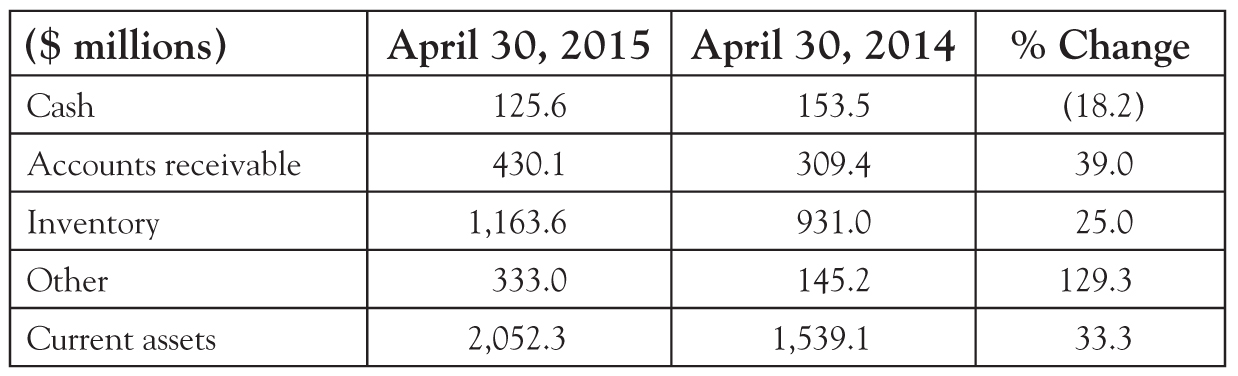
As can be seen from the previous table, current assets rose 33.3 percent, much more than the 1.4 percent increase in sales. The firm had an 18.2 percent drop in cash, which makes sense given the acquisition and additional debt incurred. Cash and other current assets combined remained about the same total dollar value as accounts receivable. Inventory is the largest item, roughly three times the size of accounts receivable. Both accounts receivable and inventory increased significantly. Why did accounts receivable increase so much more than sales (39.0 percent versus 1.4 percent)? Probably due to the acquisition. Likewise, the increase in inventory may be due to the firm stocking up on key raw materials, building up inventory for an expected increase in sales, or primarily as a result of the acquisition. These are the types of considerations a user of the annual report might have. The key point is that the reader should now be able to follow this type of discussion and understand these components of the Balance Sheet.

The next chapter will examine noncurrent assets including property, plant, and equipment; patents; trademarks; and other noncurrent assets.

_________________

¹The ordering of assets differs by country. Firms in the US and Canada normally list cash first.

²They were the largest U.S. firms by market capitalization (the market price of a share times the number of shares held by the public) as of January 29, 2016. Apple is #1 (at $542.7 billion), Alphabet (Google) is #2 (at $523.6 billion), Microsoft is #3 (at $440.1 billion), and Exxon (ExxonMobil) is #4 (at $324.1 billion).

³Bonds are discussed in detail in Chapter 9.

⁴See Apple Inc. | 2015 Form 10-K | 47.

⁵See Google Inc. | 2014 Form 10-K | 52.

⁶As an aside, one item that should not be included as a cash equivalent would be postage stamps. Just for fun, try returning them to the post office and asking for a refund. They are not easily turned into cash.

⁷See: http://news.cnet.com/2100-1001-202143.html (viewed 11/24/14 10 PM EST).

⁸However, the mark-to-market rule remains highly controversial. A more complete discussion is provided in Accounting for Fun and Profit: Understanding Advanced Topics in Accounting.

⁹Note, 2/10 n/60 translates to roughly an annual rate of 14 percent. With 2/10 n/60 a customer who properly manages its cash should pay either on Day 10 or Day 60. This means a 2 percent discount is offered for paying 50 days earlier. Because there are roughly seven 50-day periods in a year (365 / 50), this means a firm taking the discount will earn approximately 14 percent over the year (7 × 2%). If the customer’s cost of capital is less than 14 percent, she should take the discount, otherwise it is better to pay on Day 60.

¹⁰Another interesting aside is the terms of delivery. Goods are considered delivered when they are placed on the transport if the terms are free on board (FOB) but not until they reach the customers place of business if the terms are free to destination (FTD). Now consider a firm loading its product onto a ship, the terms are FOB, and the merchandise falls into the water between the dock and the ship. Are the goods considered to have been delivered? It depends on where the crane loading the goods is located. If the crane is on the dock, then the goods are not considered delivered to the ship until they are on the ship. However, if the crane is on the ship, then the goods are considered delivered as soon as the goods are lifted off the dock.

¹¹The ADA can never be more than the total A/R because it cannot reduce A/R below $0 (A/R − ADA > $0). Also, the ADA can never go below $0, it cannot increase net A/R.

¹²See http://blog.freedmaxick.com/summing-it-up/bid/130347/Allowances-for-Doubtful-Accounts (viewed November 25, 2014 2 p.m. EST).

¹³According to its annual report, Exxon had deferred tax liabilities of $36.8 billion as at December 31, 2015. See, ExxonMobil Inc. | 2015 Form 10-K | page 65. Tax payments will be discussed in more detail in Chapter 7.

¹⁴This remains true today and is, to this author’s knowledge, the only case in the U.S. where a firm tax accounting choice is linked to the firm’s public reporting choice (i.e., LIFO conformity, IRS Code 472-2(e)).

¹⁵See Gary C. Biddle and Frederick W. Lindahl, “Stock Price Reactions to LIFO Adoptions: The Association Between Excess Returns and LIFO Tax Savings,” Journal of Accounting Research Vol. 20, No. 2, Autumn 1982.

¹⁶See, Kleinbard, Edward D., George A. Plesko, and Corey M. Goodman, “Is it Time to Liquidate LIFO,” Tax Notes, Vol. 113, No. 3, pp. 237–253, October 16, 2006, and ww2.cfo.com/accounting-tax/2006/07/the-battle-to-preserve-lifo/

¹⁷The European Union required all public firms to adopt IFRS for their consolidated accounts by 2005. IFRS are those issued by the International Accounting Standards Board (IASB) an independent body based in Europe. Prior to 2001, when the IASB changed its nomenclature to IFRS, these standards were called International Accounting Standards (IAS).

¹⁸This is a simplified example because in reality, different wells would have different costs and the total amount they could be sold for would depend on the quantity of oil found and its extraction costs.

¹⁹The J.M. Smucker Company owns brands, such as Smucker’s, Folgers, JIF, Pillsbury, and Crisco, among many others. See J.M. Smucker Inc. | 2015 Annual Report |.