CHAPTER 5

Health Service Resource Management Process Design

This chapter presents a case that performs a Level iii design and does not have a previous Business Design, illustrating what we defined as local case, when design levels were presented in Chapter 2.

Here the strategic issue is to generate the best possible service by having the right capacity and determination of resources accordingly to assure a service time; the value that can be generated for patients is to improve the service in terms of waiting time and providing the right service. For this Intelligent Structure II is required, since we need predictive and resource optimization models to provide a required level of service at a minimum cost. Hence, BP6, “Optimum Resource Usage,” is applicable. Therefore from this we design a new process configuration for the service that reduces waiting time and improve service, besides evaluating them for a forecasted demand. Such design is based on representing the design problem by means of a process architecture. To do this the Shared Services Architecture Pattern, adapted to hospitals as in Figure 2.7, is used. To exemplify this design of configuration and capacity, we concentrate on the “Services Lines for Patients” in the figure, detailed in Figure 5.1, selecting the “Demand Analysis and Management” process in relation to the “Emergency Medical Service.” This process needs the subprocess of “Demand Forecasting and Characterization,” including business logic, which will be detailed in what follows.

To be able to forecast effectively, one of the key factors is the quality of historical data. In addition, the hospital operating conditions and environment should remain relatively stable for the data to be representative. This work focuses on two public pediatric hospitals: from now on referred to as HLCM and HEGC, and a general purpose hospital, HSBA. On arrival at the emergency facilities each patient is registered, including personal data, time of arrival, diagnosis, and classification according to severity of illness. All the historical data for the three hospitals was obtained for the purposes of this work and are as follows:

• HLCM: from January 2001 to December 2009

• HEGC: from January 2001 to July 2009

• HSBA: from January 2000 to December 2009

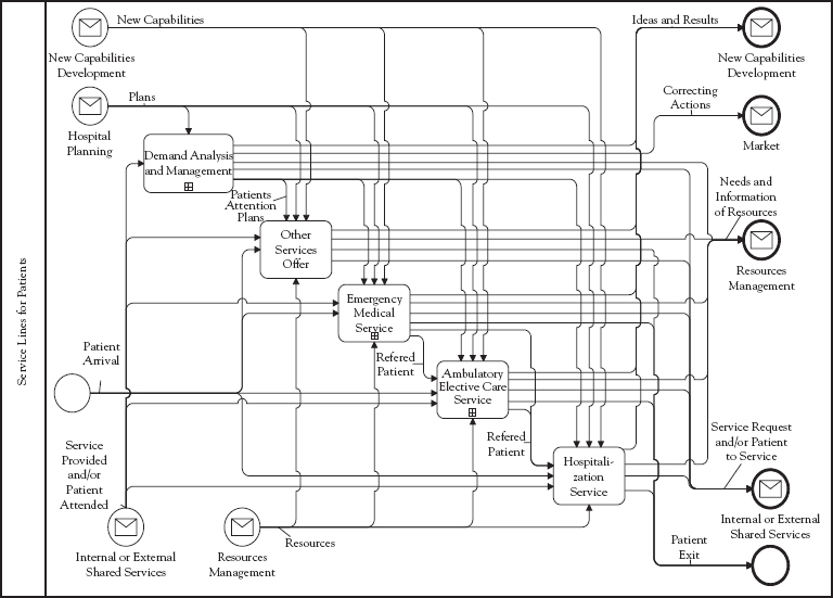
Figure 5.1 Detail of “Services Lines for Patients”

Since these hospitals could provide high-quality data regarding their emergency operation, we could infer historical demand with forecasting Analytics, reviewed in Chapter 2. We used monthly aggregated demand as a basis to construct predictive models.

However, to convert historical data into useful input information for the forecasting models, further analyses and a series of transformations were necessary. By analyzing the demand that arrives at the emergency department outliers were detected as shown in Figure 5.2. Visual inspection of aggregated demand as shown in such figure for one of the hospitals reveals a strong seasonal pattern. We observed a low demand during the summer months (December, January, and February in the Southern Hemisphere) and a high influx of patients during the winter season (May, June, and July). In general, a downward trend can be observed over the years.

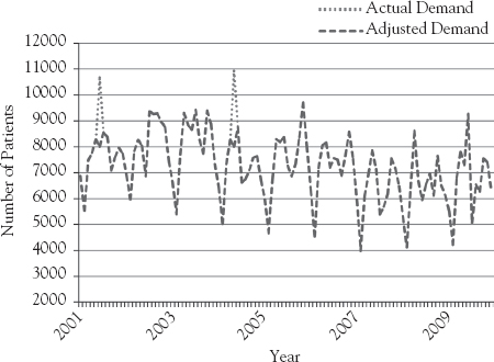
Figure 5.2 Actual versus adjusted demand per month in HLCM

When data is disaggregated by pathology type we notice huge differences, as shown for medical and surgical demand in Figures 5.3 and 5.4. The first is much more volatile over the years since it depends on factors such as temperature and flu-like illness rate, while the second is more stable over the years. We also conclude that medical demand comprises 70 percent of the emergency cases and surgical demand corresponds to 30 percent of the cases.

Demand at HEGC and HSBA shows behaviors that are very similar to the demand at HLCM. Four forecasting methods are applied: Linear Regression, Weighted Moving Averages, Neural Networks, and Support Vector Regression (SVR). The first two are well-known techniques used for forecasting and described in the literature.¹ Neural Networks and SVR are techniques that are increasingly used for forecasting.² We used Mean Absolute Percentage Error (MAPE) and Mean Square Error (MSE) as performance measures to determine model accuracy. For the Linear Regression, Weighted Moving Average, and SVR, the same inputs as the ones described for the Neural Network are used. Results obtained using these four methods for the validation sets of all hospitals are shown in Table 5.1. As observed in this, in five out of seven cases, best results are obtained with SVR, when using MSE as criterion to compare the different models’ performance. When using MAPE as criterion for comparison, SVR appears as the best option for demand forecasting in all cases.

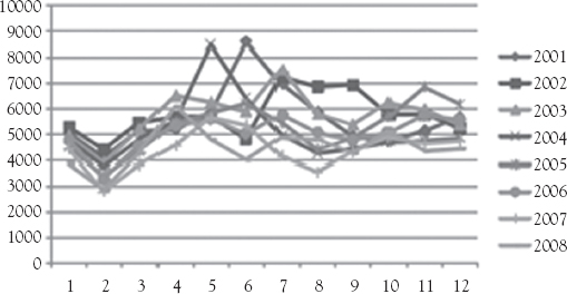
Figure 5.3 Medical demand for HLCM

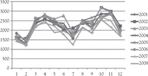
Figure 5.4 Surgical demand for HLCM

Given the results described earlier and based on the fact that SVR is built on a solid theoretical foundation, we conclude that it is the most appropriate method for predicting demand in emergency rooms. For practical use, we recommend to additionally consider using simpler methods, which produce results that can be acceptable under certain conditions.

Just having a forecast for the number of patients arriving at emergency rooms is not sufficient for capacity management; also needed are the different kinds of resources necessary to attend the patients. Following the health care conventions used in Chilean hospitals, patients are classified into four categories according to the severity of their illness, as shown in Table 5.2. Each category is associated with different uses of the medical resources, as explained in the following.

As shown in Figure 5.5, the illness severity distribution varies over the different months of a year. Nevertheless, the severity distribution per month remains relatively stable over the years. Therefore, in the following calculations, each month will be considered to have a deterministic distribution of patients for each category.

Given the emergency patients forecast and the illness severity distribution, the expected number of patients per category can be calculated. To determine the number of doctors required to attend such demand, the next step is to characterize the behavior of the attention time for each category. For this purpose, a representative sample of C1, C2, C3, and C4 individuals was used.

Each C1 patient is referred to the reanimation room for resuscitation, upon the patient’s arrival to the emergency service. When this occurs, and depending on the complexity of the surgery or diagnosis, between one and three of the doctors currently working in the attention cubicles immediately set aside their activities to focus on the extreme risk patient. After the medical attention, the time required to stabilize and treat the C1 patient is registered in a logbook, along with the names of the doctors who performed the medical procedure.

Table 5.1 Forecast errors on validation sets (best results in bold)

Table 5.2 Category types and description

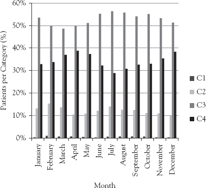
Figure 5.5 Monthly categorization distribution

Using this information, we run a K-S test to determine the distribution of the C1 patients’ attention time. We concluded that it has a log normal distribution with a mean of 108 minutes and a standard deviation of 121 minutes. We also noticed that the number of doctors required to attend these patients had a highly concentrated distribution in two doctors; therefore, this value was used for the following calculations.

When trying to characterize the consultation of C2 patients, the data used did not provide enough information to determine a distribution of the attention time. However, in a discussion with the doctors, a consensus was reached where the average time to attend C2 patients is 60 minutes, with a standard deviation of 20 minutes. A normal distribution was chosen to represent the behavior of this attention time.

Finally, and with a high level of confidence, we determined the distribution of the attention time for C3 and C4 patients as log normal with means of 10 and 7 minutes, and standard deviations of 7 and 3 minutes, respectively. All non-C1 patients are attended by only one doctor.

The time distributions presented earlier provide a basis to estimate the time that doctors will spend to attend the patients from each category, expected to arrive to the emergency room. A summary of the attention time distributions found for the different severity categories and the number of medical doctors required to attend each patient per category is presented in Table 5.3.

An analysis of patient arrivals at different times of the day was performed, as shown in Figure 5.6. This study concluded that 59 percent of the patients arrived at the emergency service between 12:00 and 20:00 hours. Using a representative sample we found that this distribution does not vary significantly among different days of the week or among the same days of different weeks. Therefore, this distribution is considered as fixed for every day of the year.

Now, given a forecast, the subprocess “Capacity Analysis” for the configuration design within the “Demand Analysis and Management” process in relation to the “Emergency Medical Service” in Figure 5.1 is needed, as explained next.

In the literature, several proposals for the configuration of emergency services are defined³ of which we selected the Option b in Figure 5.7, which considers a Triage, for patient pre-evaluation, and a fast-track line for patients that according to evaluation are more critical; this was complemented with parallel medical facilities for less urgent patients. For such a configuration we developed a simulation model, shown in Figure 5.8, which evaluates waiting time for a given demand. The simulation model incorporates the stochastic behavior of the demand. Since the waiting time and length of lines have shown to be significantly higher for medical attention, the simulation will be performed for these patients only. The forecast has an error with a normal distribution. To simulate the different demand scenarios for each month, the forecast was adjusted several times by different values sampled from the normal distribution of the error. Due to the stability of its daily behavior, the demand of each scenario was distributed uniformly across every day of the month. The daily demand was further disaggregated into hourly demand. As a consequence, we were able to generate several scenarios of monthly demand disaggregated per hour. Using the hourly forecasted demand from each of the scenarios generated as described earlier, the average forecasted demand was calculated for each hour of the day. We assumed that the hourly demand arrives according to a Poisson process; then this average corresponds to the mean of the Poisson distribution per hour.

Table 5.3 Distribution of attention time and number of physicians per category

On their arrival at the emergency service, patients are categorized and served according to the time distributions, which are also stochastic. Now that the stochastic behavior of the demand and the medical attention has been incorporated into the problem, we will discuss the construction of the simulation model and its role in the management of hospital capacity. In capacity configuration management, we want to determine how different designs of the hospital facilities, which determine the production process, may affect the quality of service, measured in length of wait (LOW) before the first medical attention. The simulation model allows us to observe how the expected flow of patients will use the different services offered in the facilities of the hospital, and how the available capacity performs when attending such demand. As a consequence, capacity can be redistributed or adjusted with the objective of eliminating bottlenecks and reducing idle resources. This provides a powerful decision tool for managing capacity in such a way that a given service level can be guaranteed at minimum cost.

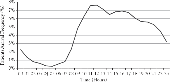
Figure 5.6 Patients’ arrival distribution per hour

As stated earlier, the average LOW will be used as the main criterion to compare the performance of the system designs. This metric was calculated weighing the demand per category by its respective average LOW. The results for this metric for the Base and Fast-Track simulated configurations are presented in Table 5.4.

On the basis of the scenarios run in the simulation, a 95-percent confidence interval was generated for the LOW of each configuration. The intervals obtained were (55.5, 59.1) and (61.8, 66.6) for the Base Case and Fast-Track with Triage, respectively. To test if the LOW differs significantly between these two configurations, we applied the procedure proposed by Law and Kelton.⁴ This comparison is established based on the difference of their respective statistical distributions, as displayed in Table 5.5. Since the confidence interval does not contain the value zero, we confirm that the difference shown is statistically significant.

On the basis of the results presented in Tables 5.4 and 5.5, we observe that:

• The simulation model resembles the actual behavior of the system, since current average LOW is within the confidence interval of the simulated Base Case.

• The main bottleneck occurs in the medical consults and during the day shift.

• The Fast-Track with Triage reduces the average LOW in 6.9 minutes, which corresponds to a 10.8-percent reduction of the current average waiting time.

• Hence, it was decided to implement the Fast-Track with Triage configuration and it was the one used in the hospital where work was performed. Another hospital is replicating the forecasting and simulation-based processes, due to the good results obtained in the first hospital.

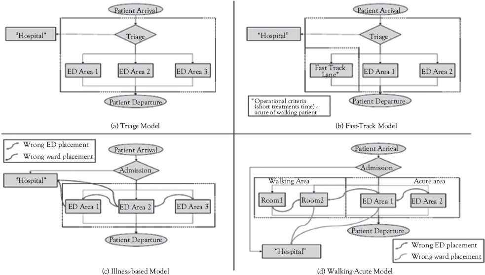
Figure 5.7 Alternative configurations for emergency services

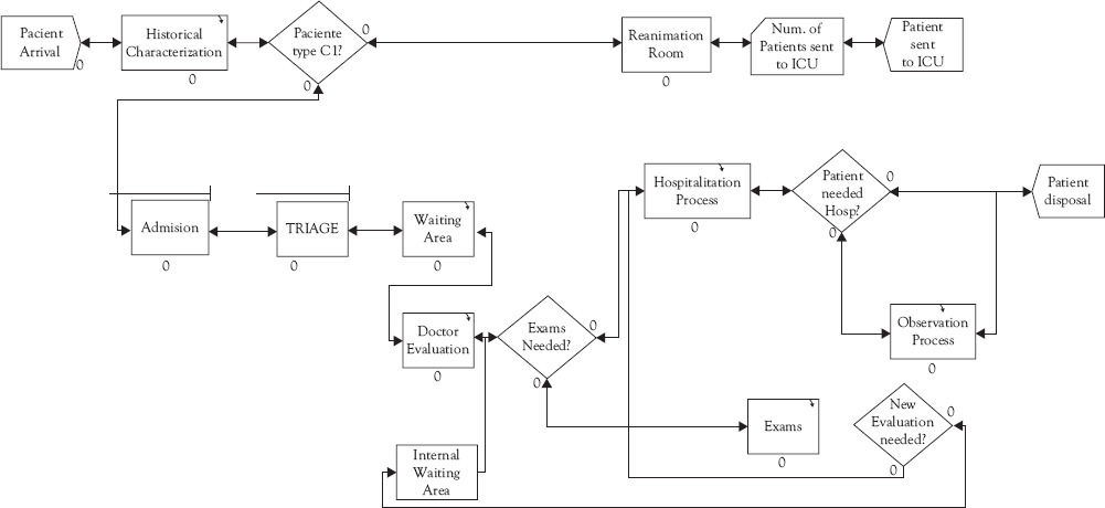
Figure 5.8 Simulation model for Capacity Analysis

Table 5.4 Simulated LOW of different emergency service configurations

Table 5.5 Base Case and Fast-Track configurations comparison

Then, using the previous models, the resource management process is designed, for which the relevant pattern is also “Demand Analysis and Management” in Figure 5.1, performed at a lower level of detail. In the previous analysis, we considered aggregated demand for configuration (which in this case also implies service production) design, and in resource management we must use disaggregated demand for the resources needed and assign them to process operation.

For forecasting demand in the first subprocess of Figure 5.1, the same models are used as in the previous analysis, but at a more disaggregated level. Then a Capacity Analysis has to be executed. Here the key resource is availability of doctors, since they are the ones who diagnose and provide treatments for emergency patients. Hence, demand has to be converted into medical hours needed of different specialties, which were determined through technical coefficients. Comparison with available resources defines lack or excess of resources, which are the basis for the determination of correcting actions; of course, there may be a feedback among these activities in order to analyze resources for given correcting actions, such as changing number or schedules of doctors. We then evaluate the impact that redistribution, reduction, or addition of medical resources would generate on the performance of the system. The resource management analysis, then, will be performed for the Fast-Track configuration only. The same simulation model of the previous section, shown in Figure 5.8 is then run for several assignments and number of doctors per shift under the Fast-Track configuration with Triage and assuming a stochastic demand.

If the current structure of two 12-hour shifts is maintained, an initial scenario would consider only redistributing the doctors available in a different manner. Given the greater arrival of patients during the day, a possible redistribution could include the reassignment of doctors from the night to the day shift. As a consequence, more doctors would attend during the day shift than at night. The average LOW of this scenario would be 45.1 minutes. Further, resource management considerations may determine the addition or reduction of medical hours for attending the patients. Since these resources are known to be quite expensive, the different scenarios were simulated by changing the existing capacity in 0.5 doctor intervals. The extra half doctor interval was included through the creation of a new shift of 6 hours, from 12:00 to 18:00, which is precisely the period in which most patients arrive at the service. Thus, the number of 6.5 doctors available means that 4 doctors attend on the day shift (8:00 to 20:00), 1 doctor on the half shift (12:00 to 18:00), and 2 doctors at night (20:00 to 8:00). The average LOW obtained with this configuration is 40.5 minutes. The simulation was run using from 5 to 7 doctors within 24 hours, and distributed as explained earlier. The idea behind analyzing the reduction of the current number of doctors is to assess whether the performance of the system is affected in a significant manner when these resources are lacking, either by management decision or by absenteeism. The average LOW for different numbers and assignments of resources are summarized in Figure 5.9, including the 95-percent confidence interval for each of the points.

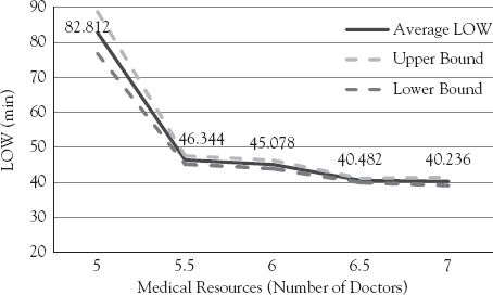
Figure 5.9 Average LOW and confidence intervals for different numbers of doctors

As expected, the addition of medical resources improves the service quality, measured in average LOW. The interesting result is that the average LOW decreases dramatically when increasing the number of medical resources from 5 to 5.5 doctors, while it decreases more gradually when new resources are added. To test whether the LOW difference between all the scenarios included in Table 5.6 is statistically significant, we applied again the procedure proposed by Law and Kelton. Table 5.6 shows the confidence intervals when comparing the LOW of these scenarios. As it can be observed, increasing from 5 to 5.5 doctors provides a significant improvement to the performance of the system, while the change between 5.5 and 6 doctors does not. Nevertheless, increasing from 5.5 to 6.5 doctors does show statistical significance.

The previous analysis of the system performance provides hospital managers a decision tool for determining the number and distribution of medical resources on the emergency service, based on a cost or benefit analysis of resources and service improvement. The previous results were used to assign doctors to the different kind of boxes and define their work schedules and also to assign additional doctors. Each of the activities of the process “Demand Analysis and Management” in Figure 5.1 has computer system support, as exemplified in the model in Figure 5.10 for “Capacity Analysis,” which uses the BPMN notation. Notice that, in order to use these tools routinely, one has to embed the models and the application logic we have described in the supporting system to the actors of the process as specified in the design of such figure.

Table 5.6 Confidence intervals for compared scenarios

It should be remarked that the process designed, with the imbedded Analytics and Information System support, is not a one-time effort. In fact, it is designed for periodically executing the whole process under changing conditions, such as unexpected demand, for example, epidemic episodes and new campaigns, which require adapting capacity.

We also notice that the process design presented includes the relationships to the other components of the Hospital Architecture. Thus, the relationship to the organizational structure is included in the process definitions, such as shared services, which is the case of “Demand Analysis and Management” of Figure 5.1, which was presented for Emergency, but needs to be coordinated with ambulatory and hospitalization and other shared services, such as surgery. We did not go into such coordination, but in a complete design it should be taken into account. If this is done it means that we are redesigning the organization as well as design the processes. Also job definition is included, since the roles in the lanes of Figure 5.10 have been assigned specific tasks in the execution of the process. IT support is specified in a very precise way as data processor and, more importantly, as a container for embedded logic that allows optimizing resource assignment. Finally, the relationships to the systems architecture and IT infrastructure should be taken into account, since the data come from current systems and the process design should be integrated with such systems. Furthermore, new technological tools, such as Analytics packages should also be integrated into the design.

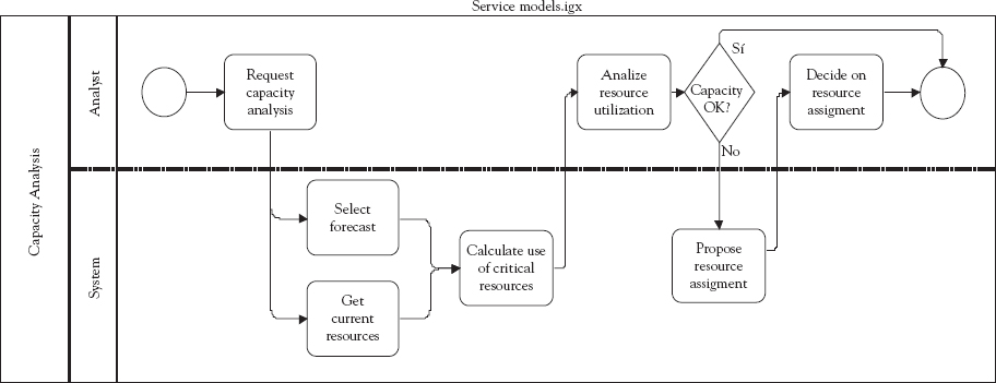
Figure 5.10 BPMN for “Capacity Analysis”