Chapter 8: Creating Data Aggregates and Metrics
8.2 Creating Simple Aggregates
8.2.1 Getting Variables from Other Tables
8.2.2 Calculating Unique Counts
8.2.3 Calculating Medians, Percentiles, Mode, and More
8.3 Creating Multi-Way Aggregates
8.3.1 Using Parameter Files to Define Aggregates
8.1 Overview
Creating data aggregates and metrics is a critical component of any business intelligence effort. Our users have asked us to provide a variety of examples that can be used by their management as well as the teams, players, and especially the fans to better understand the on-the-field performance metrics that are driving the success of the game. There is a long history of standard baseball metrics that are currently in use that they have asked us to replicate. However, they have also expressed an interest in how the SAS hash object, when combined with other SAS tools, can be used to create new metrics and perform what-if type analyses.
8.2 Creating Simple Aggregates
Our first example is calculating what is commonly referred to as a player’s slash line which is made up of the following 4 metrics:
● Batting Average (BA) – The rate a which a player gets a hit. It is calculated as the total number of hits divided by the total number of at bats (ABs). Note that baseball does distinguish between at bats and plate appearances (PAs). Every time a player goes up to home plate to hit is counted as a plate appearance. At bats exclude plate appearances where the batter reached base other than by getting a hit: for example, the batter walked, was hit by a pitch, or hit a sacrifice.
● On-Base Percentage (OBP) – The rate a which a player gets on base. The denominator in this calculation includes all plate appearances, and the numerator includes walks and hit by pitch plate appearances as well as hits (_Reached_Base in the code below).
● Slugging Percentage (SLG) – Similar to the batting average, but the numerator is the total number of bases (_Bases in the code below): a single is 1, a double is 2, a triple is 3, and a home run is 4. It is a measure of what is referred to as power hits (e.g., a double is more valuable than a single, and so on).
● On-Base Plus Slugging (OPS) – A measure that combines the power number with the frequency of getting on base and is calculated as OBP+SLG.
The following SAS program (which is also the code on the cover of the book) calculates the slash line for each player. The source data is the AtBats data (which as stated above contains one row for each plate appearance for each player).
Program 8.1 - Chapter 8 Slash Line.sas
data _null_;
dcl hash slashline(ordered:"A"); ❶
slashline.defineKey("Batter_ID"); ❷
slashline.defineData("Batter_ID","PAs","AtBats","Hits","_Bases","_Reached_Base"
,"BA","OBP","SLG","OPS"); ❸
slashline.defineDone();
format BA OBP SLG OPS 5.3; ❹
do until(lr);
set dw.AtBats end = lr; ❺
call missing(PAs,AtBats,Hits,_Bases,_Reached_Base); ❻
rc = slashline.find(); ❼
PAs + 1; ❽
AtBats + Is_An_AB;
Hits + Is_A_Hit;
_Bases + Bases;
_Reached_Base + Is_An_OnBase;
BA = divide(Hits,AtBats); ❾
OBP = divide(_Reached_Base,PAs);
SLG = divide(_Bases,AtBats);
OPS = sum(OBP,SLG);
slashline.replace(); ➓
end;
slashline.output(dataset:"Batter_Slash_Line(drop=_:)"); ![]()
run;
❶ Create the hash table and use the ORDERED argument tag so our output data set will be sorted by the player id number (which in this case is the Batter_ID field).
❷ Define the only key item for this table – the player id number. We will be adding other keys later in this chapter.
❸ Define the data items for this table. It includes both the final metrics that we want to include in our output along with the sufficient statistics that are used to do those calculations.
❹ A FORMAT statement is used so the metrics have the desired display format. Note that attributes like labels, formats, and so on are inherited by the hash variables from the corresponding PDV host variables and are carried along into the output data sets created by the OUTPUT method of the hash object.
❺ Use an explicit file-reading loop (the DoW-loop) to read all the AtBats data from the star schema data warehouse. The DW libref was defined in our autoexec.
❻ Initialize all the values we are aggregating to missing to handle the case of a Player_ID key-value not yet added to the hash table. We don’t want the PDV host variables values to persist from the previous row.
❼ The FIND method performs the direct Retrieve operation: It searches the table for the Player_ID value currently in the PDV, and, if it is found, retrieves the values of the data portion variables from the item with this key-value. If the key-value is not found, the non-key PDV host variables remain missing; if it is found, their values are overwritten with the values of the corresponding hash variables.
❽ Aggregate the values from the AtBats data. Note that the Is_A… variables are Booleans (0/1) that can simply be aggregated to the relevant count (i.e., sum) value. Note the use of the _ prefix in the variable names for those variables we do not want included in our output data set.
❾ These metrics need to be calculated only after we have read all the data for a given player. However, by calculating them here we can avoid having to add an enumeration loop using the hash iterator object. As each data row is read, the calculations are updated.
❿ The REPLACE method performs the Update All operation by overwriting the data portion variables for the items with the Player_ID values already in the table or inserting new items for the Player_ID values not already found in the table.
![]() Create an output data set with the results, once we have read all the data. Note the data set option drop=_: which excludes from the output data set any hash variable whose name begins with an underscore (_).
Create an output data set with the results, once we have read all the data. Note the data set option drop=_: which excludes from the output data set any hash variable whose name begins with an underscore (_).
Running the above program will create the following output (note that only the first 5 Player_ID values are shown).
Output 8.1 Slash Line Metrics by Player

Upon reviewing this output we can confirm that the calculations are correct, and our users have commented positively on the simplicity of the calculations. They have expressed the following requests:
● The name of the player needs to be included in the output results. In a traditional SAS program this would require additional PROC SORT and DATA steps or a PROC SQL step.
● They would also like to calculate the slash line for each team.
● They would like to include an additional metric – the number of games a player has played in.
We will address these requests in the following subsections.
8.2.1 Getting Variables from Other Tables
In order to address the first two concerns, we need to perform a table lookup operation – in other words, the Search operation, followed by the Retrieve operation to get the player’s first and last name and his team. All three of these fields are available in our Players dimension table that was created in Chapter 7. For the purposes of this first, simple example we will assume that we need to get only the player’s current name and team fields. We will present a more precise example (i.e., that deals with the possibility of players changing teams) later in this chapter.
8.2.1.1 Adding the Player Name and Team
The following program adds the player’s name and the name of his team field to our output SAS data set. Note that the changes between this program and the previous one are highlighted in bold text.
Program 8.2 - Chapter 8 Slash Line with Name.sas
data _null_;
dcl hash slashline(ordered:"A");
slashline.defineKey("Last_Name","First_Name","Batter_ID"); ❶
slashline.defineData("Batter_ID","Last_Name","First_Name","Team_SK"
,"PAs","AtBats","Hits","_Bases","_Reached_Base"
,"BA","OBP","SLG","OPS");
slashline.defineDone();
if 0 then set dw.players(rename=(Player_ID=Batter_ID)); ❷
dcl hash players(dataset:"dw.players(rename=(Player_ID=Batter_ID))" ❸
,duplicate:"replace");
players.defineKey("Batter_ID");
players.defineData("Batter_ID","Team_SK","Last_Name","First_Name");
players.defineDone();
format BA OBP SLG OPS 5.3;
do until(lr);
set dw.AtBats end = lr;
call missing(Last_Name,First_Name,Team_SK ❹
,PAs,AtBats,Hits,_Bases,_Reached_Base);
players.find(); ❺
rc = slashline.find();
PAs + 1;
AtBats + Is_An_AB;
Hits + Is_A_Hit;
_Bases + Bases;
_Reached_Base + Is_An_OnBase;
BA = divide(Hits,AtBats);
OBP = divide(_Reached_Base,PAs);
SLG = divide(_Bases,AtBats);
OPS = sum(OBP,SLG);
slashline.replace();
end;
slashline.output(dataset:"Batter_Slash_Line(drop=_:)");
run;
❶ Add fields to the definition of the slashline hash table. Using Last_Name and First_Name as the first leading variables in the composite key along with the ORDERED:"A" argument tag will result in the output data set being sorted by the player’s name.
❷ Define the player data fields to the PDV. We need to do this here so the fields are defined to the DATA step compiler before they are referenced later in this step (i.e., the CALL MISSING function).
❸ Define the hash table used to look up the needed variables and load the data using the DATASET argument tag. Since we want the current data values and we know that the dimension table is sorted in the order the rows were added for each player (by date), use the DUPLICATE argument tag, so the last row for each player is loaded into the hash table.
❹ Add fields to the CALL MISSING call routine function so that the values are not carried forward from previous rows.
❺ Use the FIND method call (unassigned since we know it cannot fail under the circumstances) to perform the Retrieve operation extracting the needed fields from the hash table.
Running the above program will create the following output (note that only the first 5 Player_ID values are shown – sorted by the player name fields).
Output 8.2 Slash Line Metrics by Player with Their Names

And as we (and you, the reader) had expected, upon reviewing this, our users asked why the team level slash lines weren’t there and why we did not add the team name to the table. We responded by pointing out that we were building up to that, and we will address both of those in the next section.
8.2.1.2 Adding Another Aggregation Level – Team Slash Lines
There are a number of approaches to adding levels of aggregation to our sample program. Our users have asked us to add slash lines at the Team level. The approach shown here will add Team and League level aggregation. It will do that by making the assumption that the aggregation is purely hierarchical. In other words, a player rolls up to one and only one team; and teams roll up to one and only one league. We know, however, that players can play for different teams; and that it is a regular occurrence for the real Bizarro Ball data, even if it is not common for our sample (generated data).
In this section, at the request of our users, we will describe an approach that assumes purely hierarchical roll-ups. Later, in the section “Creating Multi-Way Aggregates,” we will revisit this assumption and provide alternatives that do not make that assumption and allow for non-hierarchical roll-ups.
The following program illustrates this approach based on the assumption that a player rolls up to a single team and a team rolls up to a single league. As in the previous section, the changes between this program and the previous one are highlighted in bold text.
Program 8.3 - Chapter 8 Team and Player Slash Line.sas
data _null_;
dcl hash slashline(ordered:"A");
slashline.defineKey("League","Team_Name","Last_Name" ❶
,"First_Name","Batter_ID");
slashline.defineData("League","Team_Name","Batter_ID","Last_Name","First_Name"
,"PAs","AtBats","Hits","_Bases","_Reached_Base"
,"BA","OBP","SLG","OPS");
slashline.defineDone();
if 0 then set dw.players(rename=(Player_ID=Batter_ID))
dw.teams ❷
dw.leagues;
dcl hash players(dataset:"dw.players(rename=(Player_ID=Batter_ID))"
,duplicate:"replace");
players.defineKey("Batter_ID");
players.defineData("Batter_ID","Team_SK","Last_Name","First_Name");
players.defineDone();
dcl hash teams(dataset:"dw.teams"); ❸
teams.defineKey("Team_SK");
teams.defineData("League_SK","Team_Name");
teams.defineDone();
dcl hash leagues(dataset:"dw.leagues"); ❹
leagues.defineKey("League_SK");
leagues.defineData("League");
leagues.defineDone();
format BA OBP SLG OPS 5.3;
do until(lr);
set dw.AtBats end = lr;
call missing(Last_Name,First_Name,Team_SK
,PAs,AtBats,Hits,_Bases,_Reached_Base);
players.find();
teams.find(); ❺
leagues.find(); ❻
link slashline; ❽
call missing(Batter_ID,Last_Name,First_Name); ❾
link slashline;
call missing(Team_Name); ➓
link slashline;
end;
slashline.output(dataset:"Batter_Slash_Line(drop=_:)");
return;
slashline: ❼
rc = slashline.find();
PAs + 1;
AtBats + Is_An_AB;
Hits + Is_A_Hit;
_Bases + Bases;
_Reached_Base + Is_An_OnBase;
BA = divide(Hits,AtBats);
OBP = divide(_Reached_Base,PAs);
SLG = divide(_Bases,AtBats);
OPS = sum(OBP,SLG);
slashline.replace();
return;
run;
❶ Add the fields for League and Team level aggregates as both key and data portion variables in the hash table. Team_SK has been replaced by the Team_Name field.
❷ Define the League and Team data sets fields as PDV host variables.
❸ Create the hash table that will allow us to look up and extract (i.e., Retrieve) the team name.
❹ Create the hash table that will allow us to look up and extract (i.e., Retrieve) the league name.
❺ Use the FIND method (called unassigned since we know it cannot fail) to Retrieve the value for Team_Name, as well as League_SK (needed for the next lookup).
❻ Thanks to the prior lookup, we can now call the FIND method (unassigned since we know it cannot fail) to Retrieve the value for League_Name.
❼ We have moved the code to update the hash table to a LINK-RETURN section, so we can invoke it multiple times in this DATA step without replicating it. We need to run this code at the Player, Team, and League levels.
❽ Use the LINK statement to call the code that updates the Player level data in the hash object.
❾ Setting the player fields to missing allows us to create/update an item in the hash table for Team level aggregates by invoking the LINK statement.
❿ Setting the team field to missing allows us to create/update an item in the hash table for League level aggregates by invoking the LINK statement.
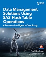
Running the above program will create the following output (note that only the first 5 rows are shown). Thanks to the ORDERED:"Y" argument tag and how missing values sort, note that the data is interleaved for us, so we see the League level numbers, then Teams within each League, and then the Players within each Team.
Output 8.3 Slash Line Metrics by League, Team, and Player

Our users liked how we did this. But users, being users, did express some concerns.
First, they were confused after looking at the complete results, that all the teams and batters seemed so similar based on their calculated slash lines. They were concerned that there was something wrong in the calculations. We had to remind them that we had used random numbers to generate the data and did not add any logic to force differences between players and teams. Once we reassured them that the program would show differences after it was run on real game data, their concern was allayed.
Second, they wanted to know how this approach handled the calculations for players who had changed teams. We clarified what we meant when we said that this approach assumed hierarchical roll-ups and that in the context of this question that meant that the entire history for a player was associated with his current team. Given the standard disclaimer that past performance is not necessarily predictive of future performance, we further suggested that the calculation of the slash line using this approach could be viewed as a best guess for what to expect at team level based on the current make-ups of the teams. And we reminded them that later in this chapter we will illustrate an alternative approach that associates the player’s performance with the team they played for at the time of each game or at bat.
Luckily, they liked this way of looking at the data and thought it might provide some interesting insights once the programs were run on the AtBats data from actual games.
8.2.2 Calculating Unique Counts
The third request that our users asked us to address was how could the count of the number of distinct games be added to the slash line calculation.
Counting the number of distinct values is something that is quite common; but it is not a standard metric included in the SAS data summarization tools dealing with additive descriptive statistics, such as the SUMMARY or the MEANS procedures. It can be calculated with other standard SAS tools, though. For example, using the SQL procedure, one can code something like:
proc sql;
create table unique as
count(distinct Game_SK) as Games
from dw.AtBats
group Player_ID;
quit;
Alternatively, the data could be sorted and then the DATA step FIRST.X/LAST.X logic could be used, such as:
proc sort data = dw.AtBats(keep=Player_ID Game_SK)
out = AtBats nodupkey;
by Player_ID Game_SK;
run;
data unique;
/* note that a DoW-loop could be used here as well */
set AtBats;
by Player_ID;
Games + 1;
If last.Player_ID;
output;
Games = 0;
run;
Most SAS programmers could come up with any number of ways to count distinct values.
Another issue with counting distinct values is that the statistic's values are not additive. In other words, you cannot add up the count of distinct games calculated at the Player_ID level to get the value at the Team or League level. Code must be written to perform that calculation at each desired level.
Fortunately, the hash object, being a keyed, in-memory table, provides an efficient and easy way to implement calculating the count of distinct values. The approach is simple:
1. Define a table that contains the current list of all the values.
2. As a new data row is encountered, check to see if the key from that row already exists in the table.
3. If the key is found, do nothing.
4. Otherwise, increment the count of distinct values by 1 and add the new value to the table, so we know that we have already encountered it.
In other words:
1. Define a hash table that has the desired grouping variables as key items.
2. Issue an assigned call to the ADD method.
3. If the item with the key-value that the ADD method accepted is found, the ADD method return code is 0, and so we do nothing.
4. Otherwise, the ADD method return code is non-zero, and so we increment our count variable by 1.
The following program adds the distinct count of Games at the Player, League, and Team level. As in the previous section, the changes between this program and the previous one are highlighted in bold text. Of particular note is how few changes were needed to add the count of distinct Games to our slash line aggregate.
Program 8.4 - Chapter 8 Slash Line with Unique Count.sas
data _null_;
dcl hash slashline(ordered:"A");
slashline.defineKey("League","Team_Name","Last_Name","First_Name","Batter_ID");
slashline.defineData("League","Team_Name","Batter_ID","Last_Name","First_Name"
,"Games","PAs","AtBats","Hits","_Bases","_Reached_Base" ❶
,"BA","OBP","SLG","OPS");
slashline.defineDone();
if 0 then set dw.players(rename=(Player_ID=Batter_ID))
dw.teams
dw.leagues;
dcl hash players(dataset:"dw.players (rename=(Player_ID=Batter_ID))"
,duplicate:"replace");
players.defineKey("Batter_ID");
players.defineData("Batter_ID","Team_SK","Last_Name","First_Name");
players.defineDone();
dcl hash teams(dataset:"dw.teams");
teams.defineKey("Team_SK");
teams.defineData("League_SK","Team_Name");
teams.defineDone();
dcl hash leagues(dataset:"dw.leagues");
leagues.defineKey("League_SK");
leagues.defineData("League");
leagues.defineDone();
dcl hash u();
u.defineKey("League","Team_Name","Batter_ID","Game_SK"); ❷
u.defineDone();
format BA OBP SLG OPS 5.3;
do until(lr);
set dw.AtBats end = lr;
call missing(Last_Name,First_Name,Team_SK,Games ❹
,PAs,AtBats,Hits,_Bases,_Reached_Base);
players.find();
teams.find();
leagues.find();
link slashline;
call missing(Batter_ID,Last_Name,First_Name,Games); ❹
link slashline;
call missing(Team_Name,Games); ❹
link slashline;
end;
slashline.output(dataset:"Batter_Slash_Line(drop=_:)");
return;
slashline:
rc = slashline.find();
Games + (u.add() = 0); ❸
PAs + 1;
AtBats + Is_An_AB;
Hits + Is_A_Hit;
_Bases + Bases;
_Reached_Base + Is_An_OnBase;
BA = divide(Hits,AtBats);
OBP = divide(_Reached_Base,PAs);
SLG = divide(_Bases,AtBats);
OPS = sum(OBP,SLG);
slashline.replace();
return;
run;
❶ Add the variable Games which will be the count of unique games played to our hash table.
❷ Create a hash table that has the same keys as our slashline hash table, with the addition of the Game_SK variable. This creates a hash table whose keys represent the list of unique combinations of League, Team_Name, Batter_ID, and Game_SK. Note that since the fields Last_Name and First_Name do not contribute to the uniqueness constraint they need not be included here. They are included only as keys in the slashline hash table in order to have the output SAS data set sorted by the player name.
❸ If the return code from the ADD method is 0, that means that this is a new combination of League, Team_Name, Batter_ID, and Game_SK. Thus, we need to increment the value of the variable Games.
❹ Add the Games variable to the CALL MISSING routine, so it is initialized before linking to the section that includes the calculations including the incrementing of the Games fields. The first call to the link section increments the Games field by 1 if the Game_SK value is new at the Player_ID level. The second call to the link section increments the Games field by 1 if the Game_SK value is new at the Team_Name level. The third call to the link section increments the Games field by 1 if the Game_SK value is new at the League level.
Running the above program will create the following output (note that only the first 5 rows are shown). Thanks to the ORDERED:"Y" argument tag and how missing values sort, note that the data is interleaved
for us, so we see the League level numbers, then teams within each league and then the players within each team.
Output 8.4 Slash Line Metrics Including Count of Unique Games

Since we know that there are 16 teams in each league and each team plays each other 12 times, the values of the Games field at the Team Level (12*15=180) and at the League level (each game involves two teams (180*16/2=1440)) are exactly what we have expected.
8.2.3 Calculating Medians, Percentiles, Mode, and More
Calculating percentiles (including the median) and the mode are supported by PROC UNIVARIATE. And, of course, custom code can be written to calculate these metrics. Anticipating that there will be requests for such metrics, we proceeded to determine how to calculate these metrics using the hash object in the DATA step. Having these values available in the DATA step, so they can be integrated with other calculations, will certainly find some use cases.
Tabulating the list of unique values that was needed in order to count the number of distinct values triggered the light bulb with an idea for how to simply calculate the median. We can merely create a hash table that contains all the values. So let us look at the program that does just this to calculate the median of the field Distance which is a measure of the distance from home plate for each hit.
Program 8.5 - Chapter 8 Median.sas
data _null_;
dcl hash medianDist(dataset:"dw.AtBats(where=(Distance > 0))" ❶
,multidata:"Y"
,ordered:"A");
medianDist.defineKey("Distance");
medianDist.defineDone();
dcl hiter iterM("medianDist"); ❷
iterM.first(); ❸
do i = 1 to .5*medianDist.num_items - 1;
iterM.next(); ❹
end;
/* could add logic here to interpolate if needed */
put "The Median is " Distance; ❺
stop;
set dw.AtBats(keep=Distance);
run;
❶ Define a hash table and load it with all the positive values of Distance. Distance can be 0 or missing for the results of at bats that did not result in a hit. The MULTIDATA:"Y" argument tag makes sure all the values are loaded into the table; the ORDERED argument tag forces the values to be inserted in sorted order by Distance.
❷ Since we need to get to the hash item corresponding to the half-way point, we need a hash iterator to do that.
❸ The hash iterator needs to be set to point inside the table. We decided to use the FIRST method to point to the first item.
❹ Use the hash iterator to loop through the hash table to get to the midpoint. We use the NUM_ITEMS attribute to determine how many items the hash table has, multiply that value by .5, and then subtract 1 since we have already pointed to the first row. So after the i=1 loop iteration we are pointing to the second row in the hash table (and so on).
❺ For this Proof of Concept (PoC) we just write the value to the log. Also note that for the purposes of this PoC we have decided not to worry about interpolating between two values for the case when the number of rows is even. That is a nuance that our business users agreed could be dealt with later.
Running the above program will create the following output in the SAS log.
NOTE: There were 209970 observations read from the data set DW.ATBATS.
WHERE Distance>0;
The Median is 204
NOTE: DATA statement used (Total process time):
real time 0.24 seconds
cpu time 0.12 seconds
A sample use case for this might be to use the median value to filter or subset the data in our current DATA step program.
8.2.3.1 Calculating Multiple Medians
Whenever we calculate metrics, we almost always need to calculate more than one metric. For example, we might want to also calculate the median value of the Direction field which measures the angle of the hit relative to home plate and the baseline. Alternatively, perhaps we want to calculate and compare the median distances for the different types of hits (e.g., singles, doubles, triples, home runs).
Using the approach shown above we would need a separate hash table for each required median that we wish to calculate. That could quickly escalate to the point where we have to create a lot of hash tables, which requires lots of code and perhaps too much memory.
Our first thought is to create four hash tables (e.g., single, double, triple, homerun) and four hash iterators (e.g., singleIter, doubleIter, tripleIter, homerunIter) and use arrays to loop through them. Arrays are commonly used when we need to perform the same operation on multiple variables – by simply looping through them. We expected that looping through our hash objects using an array would be a simple way to address this.
Program 8.6 Chapter 8 Multiple Medians Array Error.sas
data _null_;
dcl hash single(dataset:"dw.AtBats (where=(Result='Single'))" ❶
,multidata:"Y",ordered:"A");
single.defineKey("Distance");
single.defineDone();
dcl hiter singleIter("single");
.
.
.
array _hashes(*) single double triple homerun; ❷
array _iters(*) singleIter doubleIter tripleIter homerunIter;
stop;
❶ Define the hash table for singles just as in the prior example. Comparable code is used (but not shown here) for doubles, triples, and home runs.
❷ Define the arrays needed to loop through the hash objects and their respective iterators.
The SAS log resulting from this approach highlights that is not an option.
670 array _hashes(*) single double triple homerun;
ERROR: Cannot create an array of objects.
ERROR: DATA STEP Component Object failure.
Aborted during the COMPILATION phase.
NOTE: The SAS System stopped processing this step because of errors.
NOTE: DATA statement used (Total process time):
real time 0.03 seconds
cpu time 0.01 seconds
671 array _iters(*) singleIter doubleIter tripleIter homerunIter;
At first we were surprised at this error. But then realized that it made sense since neither a hash object, nor a hash iterator create numeric or character variables. As the error implies, they are objects (e.g., pointers to memory locations) as was discussed in Part 1.
Since we are just exploring this requirement as a PoC, for now we just present a simple example that calculates the median for each type of hit by repeating the code to create the hash objects and their iterators. Should our users decide to proceed with a follow-on effort we pointed out that we could use the macro language to minimize hard-coding. We also told them that an alternative to looping through multiple hash object would be described Chapter 9 Hash of Hashes – Looping Through SAS Hash Objects.
The following program illustrates an approach as an interim hard-coded solution that takes advantage of the LINK statement in the DATA step. The LINK statement is a useful feature that allows us to repeatedly execute the same block of code multiple times in a given DATA step; but without having to cut and paste the code into multiple locations.
Program 8.7 - Chapter 8 Multiple Medians.sas
data Medians;
length Type $12;
keep Type Distance Count;
format Count comma9.;
dcl hash h(); ❶
h = _new_ hash(dataset:"dw.AtBats(where=(Result='Single'))"
,multidata:"Y",ordered:"A");
h.defineKey("Distance");
h.defineDone();
type = "Singles";
dcl hiter iter; ❷
iter = _new_ hiter("h");
link getMedians; ❸
h = _new_ hash(dataset:"dw.AtBats (where=(Result='Double'))" ❶
,multidata:"Y",ordered:"A");
h.defineKey("Distance");
h.defineDone();
type = "Doubles";
iter = _new_ hiter("h"); ❷
link getMedians; ❸
h = _new_ hash(dataset:"dw.AtBats(where=(Result='Triple'))" ❶
,multidata:"Y",ordered:"A");
h.defineKey("Distance");
h.defineDone();
type = "Triples";
iter = _new_ hiter("h"); ❷
link getMedians; ❸
h = _new_ hash(dataset:"dw.AtBats(where=(Result='Home Run'))" ❶
,multidata:"Y",ordered:"A");
h.defineKey("Distance");
h.defineDone();
type = "Home Runs";
iter = _new_ hiter("h"); ❷
link getMedians; ❸
stop;
getMedians:
Count = h.num_items; ❹
iter.first(); ❺
do i = 1 to .5*Count - 1;
iter.next();
end;
/* could add logic here to interpolate if needed */
output; ❻
h.delete(); ❼
return;
set dw.AtBats(keep=Distance); ❽
run;
❶ Create an instance of hash object H for each of the four types of hits we want to calculate the median of. By using the _NEW_ operator to create a new hash object instance, we can reuse the same name for the hash object. That facilitates reusing the same code to do the median calculation.
❷ Create the requisite corresponding instances of hash iterator object ITER. Just as for the hash object creation, use the _NEW_ operator.
❸ Use the LINK statement to branch to the code that does the actual calculation of the medians. The RETURN statement at the end of the LINK block returns control to the statement after the LINK statement.
❹ Use the NUM_ITEMS attribute to get the number of items in the hash table. By assigning that value to a SAS numeric variable, we can include in the output the number of hits of each type.
❺ Use the same DO loop construct as in the Program 8.5 to get to the midpoint of the number of items. That value for the distance from the midpoint item (subject to the interpolation comment above) is the median.
❻ Once we have determined the median value, output the value to a SAS data set.
❼ While not necessary for the program to run (since these hash tables are reasonably small), using the DELETE method frees up the memory (as would the CLEAR method), making it available for the rest of the DATA step. This could be important if there are lots of medians to calculate when combined with lots of distinct values.
❽ Tell the DATA step compiler to create the PDV host variables with the same names as the hash variables defined via the DEFINEKEY and DEFINEDATA methods.
Running the above program will create the following output.
Output 8.5 Multiple Medians Values

8.2.3.2 Calculating Additional Percentiles
Recognizing that the median is simply the 50th percentile allows us to generalize the simple program above so it is not hard-coded for the 50th percentile as well as to allow for multiple percentiles. Given that we have
a hash table that has all the values in sorted order, we just need to tweak the code so it can step through the desired percentiles in order and identify which item in the hash table represents that same percentile.
The following program does that.
Program 8.8 - Chapter 8 Percentiles.sas
data Percentiles;
keep Percentile Distance; ❶
format Percentile percent5.;
dcl hash ptiles(dataset:"dw.AtBats (where=(Distance gt 0))" ❷
,multidata:"Y",ordered:"A");
ptiles.defineKey("Distance");
ptiles.defineDone();
dcl hiter iterP("ptiles"); ❸
array _ptiles(6) _temporary_ (.5 .05 .1 .25 .75 .95); ❹
call sortn(of _ptiles(*));
num_items = ptiles.num_items; ❺
do i = 1 to dim(_ptiles); ❻
Percentile = _ptiles(i);
do while (Counter lt Percentile*num_items); ❼
Counter + 1; ❽
iterP.next();
end;
/* could add logic here to read
next value to interpolate */
output; ❾
end;
stop;
set dw.AtBats; ➓
run;
❶ Specify the variables (and format) for the variables to be included in the output data set.
❷ Define the hash table to contain all the values for the subject variable (Distance) in ascending order just as in the above example that calculated the median.
❸ Define the needed hash iterator.
❹ Specify the desired percentiles using an ARRAY. Note that the values are not in the needed sort order (we added this wrinkle as one of the key IT users asked if the values needed to be specified in sort order). Since they are needed in ascending order, use the SORTN call routine to ensure the values are in sorted order. The SORTN call could be omitted if we could safely assume that the values were listed in ascending order.
❺ Get the number of items in the list so we can use that to determine which row number corresponds to the value for the desired percentile.
❻ Loop through the percentiles in order.
❼ This loop is similar to the loop used for the median calculation. We use the NEXT method to step through the data, stopping when we have gotten to the row number corresponding to that percentile (subject to the same interpolation comment as discussed above).
❽ The Counter variable keeps track of how many rows have been read so far. That allows us to avoid restarting from the first row for each desired percentile.
❾ Once we have reached the hash item for the current percentile, the value of the PDV host variable is the value of the Distance variable for that item. So we output the values to our data set.
❿ As in the above example, a SET statement after the STOP statement is used for parameter type matching- i.e., to define the needed host variables to the PDV.
Running the above program will create the following output.
Output 8.6 Multiple Percentiles

Enhancing this program to deal with multiple variables will be addressed in Chapter 9 Hash of Hashes – Looping Through SAS Hash Objects.
8.2.3.3 Calculating the Mode
The definition of the mode statistic is the value in the data that occurs most often. In order to calculate the mode, we need to know how many times each distinct value occurs. So, unlike the median which has one row for each individual value in our hash table, our hash table should contain one row for each distinct value along with a count for how many times that values was encountered. Another structural difference between the mode and the other metrics we’ve examined so far is that there can be multiple values for the mode.
The following program will determine the mode for Distance, our metric of interest.
Program 8.9 - Chapter 8 Mode.sas
data Modes;
keep Distance Count;
format Distance Count comma5.; ❶
dcl hash mode(); ❷
mode.defineKey("Distance"); ❸
mode.defineData("Distance","Count"); ❹
mode.defineDone();
dcl hiter iterM("mode"); ❺
do until(lr);
set dw.AtBats(keep=Distance) end=lr; ❻
where Distance gt .;
if mode.find() ne 0 then Count = 0; ❼
Count + 1; ❽
mode.replace(); ❾
maxCount = max(Count,maxCount); ➓
end;
do i = 1 to mode.num_items; ![]()
iterM.next(); ![]()
if Count = maxCount then output; ![]()
end;
stop;
run;
❶ Specify the variables (and format) for the variables to be included in the output data set.
❷ Define the hash table to contain all the values for the subject variable (Distance). Note that the MULTIDATA argument tag is not specified, as we want to have only one hash table item for each distinct value of Distance; likewise, the ORDER argument tag is not specified, as the internal order of the Distance values is not relevant to calculating the mode.
❸ Define the Key variable. We want only one item for each distinct value of Distance.
❹ Define the Data variables. The Count variable will be used to determine how many times each value of Distance occurs in the data. As mentioned above, the definition of the mode statistic is the value in the data that occurs most often. The desired output is the Distance value (or values) with the largest value of Count; we need to include Distance as a data variable so its value can be included in the output data set.
❺ We will need a hash iterator to perform the Enumerate All operation- i.e., to loop through all the items in the hash table, so that we can find all the Distance value(s) that are the mode.
❻ Use a DoW-loop to read the data, reading only those data observations where Distance has a value.
❼ If the value of Distance for the PDV host variable is not found in the hash table, initialize the Count variable to 0; if the value is found, the PDV host variable (COUNT) is updated using the hash variable value.
❽ Increment the Count variable.
❾ The REPLACE method will add the item to the hash table if it is not already found (with a value of 1 for Count); otherwise it will update the current item with the incremented value of COUNT in the hash table.
❿ As we read the data, determine what the largest value of Count is. Once we have read all the data, all the Distance items with that value for Count are mode values.
![]() Loop explicitly through the hash table using the hash iterator.
Loop explicitly through the hash table using the hash iterator.
![]() Use the NEXT method to retrieve the Distance and Count values for the current item.
Use the NEXT method to retrieve the Distance and Count values for the current item.
![]() Output a row to our output SAS data set for every Distance value that has the maximum value for Count.
Output a row to our output SAS data set for every Distance value that has the maximum value for Count.
Running the above program will create the following output. Note that we have two values of Distance which are the mode.
Output 8.7 Modes for the Variable Distance

8.2.3.4 Calculating Percentiles, Mode, Mean, and More in a Single DATA Step
As expected, our users liked the simplicity of the samples to calculate these metrics. But they commented that it would be even better if we could combine all of these calculations into a single program (which we interpreted as a single DATA step program) that could be used as template or starter program. For example:
● Removing calculations that they are not interested in for a given analysis or report.
● Adding other calculations like, for example, the interquartile range.
● Combining multiple metrics in order to create a filter. For example, looking at the distribution of the kinds of hits where the Distance is between the mean and median.
● Various What-If analyses such as the variability of these results by factors such as home vs. away team.
● And so on, and so on.
We responded by thanking them for leading us into the very next example that we had already planned to present; while reminding them that our plan is to generalize and parameterize these programs- perhaps later in this Proof of Concept (Chapter 9) or as part of an implementation project.
The following program not only combines the calculation of the mean, median and the mode into a single DATA step, it also integrates the calculation of percentiles as well as a complete frequency distribution. As such, we warned both the IT and business users that it likely would take some time to fully understand it.
Program 8.10 - Chapter 8 MeanMedianMode.sas
%let Var = Distance; ❶
data ptiles; ❷
input Ptile;
Metric = put(Ptile,percent6.); ❸
retain Value . ;
datalines;
.05
.1
.25
.5
.75
.95
;
data _null_;
format Percent Cum_Percent percent7.2;
dcl hash metrics(dataset:"ptiles" ❹
,multidata:"Y"
,ordered:"A");
metrics.defineKey("Ptile");
metrics.defineData("Ptile","Metric","Value");
metrics.defineDone();
dcl hiter iterPtiles("metrics"); ❺
dcl hash distribution(ordered:"A"); ❻
distribution.defineKey("&Var");
distribution.defineData("&Var","Count","Percent","Cumulative","Cum_Percent");
distribution.defineDone();
dcl hiter iterDist("distribution"); ❼
do Rows = 1 by 1 until(lr); ❽
set dw.AtBats(keep=&Var) end=lr;
where &Var gt .;
if distribution.find() ne 0 then Count = 0; ❾
Count + 1; ➓
distribution.replace(); ![]()
Total + &Var; ![]()
maxCount = max(Count,maxCount);
end;
iterPtiles.first(); ![]()
last = .;
do i = 1 to distribution.num_items; ![]()
iterDist.next();
Percent = divide(Count,Rows); ![]()
_Cum + Count; ![]()
Cumulative = _Cum;
Cum_Percent = divide(_Cum,Rows);
distribution.replace(); ![]()
if Count = maxCount then metrics.add(Key:.,Data:. ,Data:"Mode",Data:&Var); ![]()
if last le ptile le Cum_Percent then ![]()
do; /* found the percentile */
Value = &Var;
if ptile ne 1 then metrics.replace(); ![]()
if iterPtiles.next() ne 0 then ptile = 1;
end; /* found the percentile */
last = Cum_Percent; ![]()
end;
metrics.add(Key:.,Data:.,Data:"Mean",Data:divide(Total,Rows)); ![]()
iterDist.first(); ![]()
metrics.add(Key:.,Data:.,Data:"Min",Data:&Var);
iterDist.last(); ![]()
metrics.add(Key:.,Data:.,Data:"Max",Data:&Var);
metrics.output(dataset:"Metrics(drop=ptile)"); ![]()
distribution.output(dataset:"Distribution"); ![]()
stop;
set ptiles; ![]()
run;
❶ A macro variable is used to specify the variable to be analyzed. We wanted to introduce our users to leveraging other SAS facilities like the macro language.
❷ Likewise, we wanted to start illustrating the advantages of parameterizing (e.g., using data-driven approaches) our programs by reading in data values like the percentile values to be calculated.
❸ The variable Metric is created as a character variable so our DATA step can assign character values for other metrics to be calculated (e.g., “Mean”).
❹ Define our hash table and load the data using the DATASET argument tag. The ORDERED option is used to ensure that the percentiles are loaded in ascending order as that is needed to support the calculation of the percentiles using the same logic as in the above programs. We set the MULTIDATA argument tag to “Y” since we are calculating other metrics and will set the value of the ptile variable to values like "Mean", "Median", etc., for those other metrics.
❺ A hash iterator is needed so we can loop through (i.e., enumerate) the percentile values in the metrics hash table.
❻ Create the hash table which will tabulate the frequency distribution (including the cumulative count) of the analysis variable values. The calculation of the mode requires that we create this table so it has one item per distinct value of our analysis variable. The ORDERED argument tag is needed so we can calculate the cumulative counts and percentages as well as the specified percentiles.
❼ A hash iterator is needed so we can loop through (i.e., enumerate) the values in the distribution hash table.
❽ This form of the DoW-loop allows us to loop through all the input data in a single execution of the DATA step and have a value for the Rows variable that is the number of observations read from the input data set.
❾ If the current value of our analysis variable is not found as a key in our Distribution hash table, we initialize the PDV host variable Count to 0; otherwise, if it is found, the value of the Count variable from our hash table updates the value of the PDV host variable.
❿ Increment the value of the PDV host Count variable by 1.
![]() Use the REPLACE method to update (or add an item) to our hash table.
Use the REPLACE method to update (or add an item) to our hash table.
![]() The Total and Maxcount variables are needed, respectively, so we can calculate the mean and determine the mode values.
The Total and Maxcount variables are needed, respectively, so we can calculate the mean and determine the mode values.
![]() Once we have read all the data and have the frequency count, get the first (which due to the ORDERED:”A” argument tag is the smallest one) percentile to be calculated and assign a value to the variable last which we will use to keep track of the previous cumulative percent.
Once we have read all the data and have the frequency count, get the first (which due to the ORDERED:”A” argument tag is the smallest one) percentile to be calculated and assign a value to the variable last which we will use to keep track of the previous cumulative percent.
![]() Use a DO loop to enumerate through the values of the distribution hash table. Each time through the loop use the NEXT method to advance the hash pointer (on the first execution of the loop the NEXT method points to the first item).
Use a DO loop to enumerate through the values of the distribution hash table. Each time through the loop use the NEXT method to advance the hash pointer (on the first execution of the loop the NEXT method points to the first item).
![]() Calculate the percentage for the current item by dividing Count by Rows (the total number of observations).
Calculate the percentage for the current item by dividing Count by Rows (the total number of observations).
![]() Since Cumulative is in the hash table, the NEXT method will overwrite the PDV host variable with a missing value (since we have not yet calculated it). So we use a temporary variable, _Cum, to accumulate the running total and then assign the values to the Cumulative PDV host variable followed by the calculation of the cumulative percentage.
Since Cumulative is in the hash table, the NEXT method will overwrite the PDV host variable with a missing value (since we have not yet calculated it). So we use a temporary variable, _Cum, to accumulate the running total and then assign the values to the Cumulative PDV host variable followed by the calculation of the cumulative percentage.
![]() Use the REPLACE method to update the variables in the distribution hash table with the values of Cumulative and Cum_Percent.
Use the REPLACE method to update the variables in the distribution hash table with the values of Cumulative and Cum_Percent.
![]() If the current value of our analysis variable is equal to the largest value, it is a mode value. Therefore, add a row to our hash table of results, metrics. Note that multiple mode values are possible. We use an explicit ADD method with a value of missing for ptile. This forces the ptile value to be inserted before the percentile values are already there. This has two desirable effects: the item is added before the current pointer value and so our NEXT method calls will not encounter them; the items are added to the hash table metrics in order within the value for the key which has a missing value.
If the current value of our analysis variable is equal to the largest value, it is a mode value. Therefore, add a row to our hash table of results, metrics. Note that multiple mode values are possible. We use an explicit ADD method with a value of missing for ptile. This forces the ptile value to be inserted before the percentile values are already there. This has two desirable effects: the item is added before the current pointer value and so our NEXT method calls will not encounter them; the items are added to the hash table metrics in order within the value for the key which has a missing value.
![]() If the current percentile that we are calculating is between the previous and current cumulative percent, the value of the analysis variable is our percentile value. Note that, as mentioned above, we could add interpolation logic. That level of precision is not needed in our PoC.
If the current percentile that we are calculating is between the previous and current cumulative percent, the value of the analysis variable is our percentile value. Note that, as mentioned above, we could add interpolation logic. That level of precision is not needed in our PoC.
![]() Our program needs to loop through the entire distribution, including those values beyond the largest desired percentile. These two statements do that. We update the hash table with the value for the current percentile as long as it is not the value of 1 (it is assigned by the next statement). The NEXT method advances to the next item in our metrics hash table to get the next percentile to be calculated. If there are no more percentiles, we assign a value of 1 (i.e., 100%) to force processing of the remaining rows in the distribution hash table.
Our program needs to loop through the entire distribution, including those values beyond the largest desired percentile. These two statements do that. We update the hash table with the value for the current percentile as long as it is not the value of 1 (it is assigned by the next statement). The NEXT method advances to the next item in our metrics hash table to get the next percentile to be calculated. If there are no more percentiles, we assign a value of 1 (i.e., 100%) to force processing of the remaining rows in the distribution hash table.
![]() Assign the current cumulative percentage to the last variable so it can be used in the comparison the next time through the loop.
Assign the current cumulative percentage to the last variable so it can be used in the comparison the next time through the loop.
![]() Add the mean to the metrics hash table. Note that since we use an explicit ADD method to assign missing values to the argument tags, the item is added to the hash table in order.
Add the mean to the metrics hash table. Note that since we use an explicit ADD method to assign missing values to the argument tags, the item is added to the hash table in order.
![]() Use the FIRST method to get the value for the first item. By definition that is the minimum value. It is added to the metrics hash table (in order).
Use the FIRST method to get the value for the first item. By definition that is the minimum value. It is added to the metrics hash table (in order).
![]() Use the LAST method to get the value for the last item. By definition that is the minimum value. It is added to metrics hash table (in order).
Use the LAST method to get the value for the last item. By definition that is the minimum value. It is added to metrics hash table (in order).
![]() Use the OUTPUT method to output our calculated metrics. Note that the ptile variable is dropped because we have the character representation of the value.
Use the OUTPUT method to output our calculated metrics. Note that the ptile variable is dropped because we have the character representation of the value.
![]() Use the OUTPUT method to output the complete distribution.
Use the OUTPUT method to output the complete distribution.
![]() As in a number of the previous examples, a SET statement after the STOP statement is used to define the needed variables to the PDV.
As in a number of the previous examples, a SET statement after the STOP statement is used to define the needed variables to the PDV.
Running the above program will create the following output data sets. Note that we have printed only the first 10 observations for the complete distribution.
Output 8.8 The Metrics Data Set


Output 8.9 The Distribution Data Set – First 10 Rows

8.2.3.5 Determining the Distribution of Consecutive Events
Our users have now asked us to provide another example. They would like to determine how many times a team gets at least 1, 2, 3, or more hits in row. And they would also like to calculate a variation of that – how many times do we see exactly 1, 2, 3, or more hits in the row. The distinction between these is that, for example, 4 consecutive hits can be treated differently:
● If we are determining the distribution of at least N consecutive events, then 4 hits in a row would contribute a count of 1 to each of 1, 2, 3, and 4 hits in row.
● If we are determining the distribution of exactly N consecutive events, then 4 hits in a row would contribute a count of 1 to just the case of 4 hits in row.
At first glance, the first calculation seems to be somewhat easier to determine as we don’t need to look ahead to see if the next at bat results in a hit. However, since the number of consecutive events is calculated, if the next at bat is not the same event, the number of consecutive events is not updated. The logic is actually calculating how many times we have exactly N consecutive events. We can then use those values to calculate N or more consecutive events.
In statistical terminology, what we are describing here as “consecutive events” is often referred to as a run which is defined as a series of increasing values or a series of decreasing values. It is a given that the term run has a well-defined meaning in baseball which is different from this definition. Thus, we will continue to refer to this as “consecutive events” even though it is indeed a run in statistical terminology.
Such calculations are something that could be done with a DATA step to calculate the value for N, followed by, for example, the FREQ procedure to get the distribution. However, given the example in the
previous section, we know that we can create a frequency distribution in a DATA step using the hash object. Our DATA step hash table approach needs to:
● Calculate the value for the number of consecutive hits.
● Count how many times each value occurs (that gives us the count for that many or more).
● Calculate the count for how many times we see exactly N consecutive events.
● Output the results to an output SAS data set.
We decided that the SUMINC argument tag could be used to do this. The SUMINC argument tag is used on the DECLARE statement or with the _NEW_ method. The value provided for this argument tag is a character expression which is the name of a DATA step variable whose value is to be aggregated. This variable is not included as a data variable in the hash table; instead memory is allocated to accumulate (i.e., sum) the value of the designated variable behind the scenes.
There are two issues to be aware of when using SUMINC: first, only one variable can be summed; second, a METHOD call is needed to retrieve the value – it is not explicitly linked or tied to a PDV host variable. For our current example, neither of these is an issue, as can be seen in the following program which calculates the distribution of consecutive hits.
Program 8.11 - Chapter 8 Count Consecutive Events.sas
data Consecutive_Hits;
keep Consecutive_Hits Exact_Count Total_Count;
format Consecutive_Hits 8.
Exact_Count Total_Count comma10.;
retain Exact_Count 1; ❶
if _n_ = 1 then
do; /* define the hash table */
dcl hash consecHits(ordered:"D",suminc:"Exact_Count"); ❷
consecHits.defineKey("Consecutive_Hits"); ❸
consecHits.defineDone();
end; /* define the hash table */
Consecutive_Hits = 0;
do until(last.Top_Bot); ❹
set dw.atbats(keep=Game_SK Inning Top_Bot Is_A_Hit) end=lr;
by Game_SK Inning Top_Bot notsorted;
Consecutive_Hits = ifn(Is_A_Hit,Consecutive_Hits+1,0); ❺
if Is_A_Hit then consecHits.ref(); ❻
end;
if lr; ❼
Total_Adjust = 0; ❽
do Consecutive_Hits = consecHits.num_items to 1 by -1; ❾
consecHits.sum(sum:Exact_Count); ➓
Total_Count = Exact_Count + Total_Adjust; ![]()
output;
Total_Adjust + Exact_Count;
end;
run;
❶ Assign a value of 1 to the variable we will use as the value of the SUMINC argument tag. Since we are counting events, the value to be added to our sum (which is a count) is always 1.
❷ Define the hash table. We used ORDERED:”D” for two reasons. One, in order to calculate the count of N or more events we need the table to be ordered; and two, we want the output sorted by the descending count of consecutive events. Note also that these statements are executed only on the first execution of the DATA step. This is the first sample in this chapter for which our DATA step executes multiple times and so, unlike earlier examples, we need to add logic so the Create operation (defining and instantiating the hash table) is performed only once – on the first execution of the DATA step.
❸ Define the key to be the number of consecutive events. Note that since we do not have a DEFINEDATA method call, the same variable is automatically added to the data portion of the hash table. Since SUMINC is used to do the aggregation, no other variables are needed in the data portion.
❹ We use a DoW-loop coupled with the BY statement, so each execution of the DATA step reads the data for a single half-inning. We don’t want our consecutive events to cross half-inning boundaries. The variable Consecutive_Hits is initialized to 0 since we want to restart our count for each half-inning.
❺ The IFN function is used to either increment our counter of consecutive events if the current observation represents a hit or to reset it to 0 if not. In response to a question from one of the IT users we confirmed that the IFN function has an optional fourth argument if the first argument has a null or missing value. Our use case does not have to handle null/missing values.
❻ When using SUMINC, the REF method (discussed in Part 1) should be used to keep the value of the PDV host variable and the hash table data item in synch. We need to do this only when we have consecutive events which caused the PDV host variable to be incremented by 1.
❼ Once we have read all the data, we are ready to post-process our hash table to create an output data of the distribution.
❽ Initialize the variable we use to increment the count of exactly N events to calculate N or more events.
❾ We can enumerate the hash table since we know the number of consecutive events will always be a sequence of integers starting with a value of 1 and incremented by 1. Thus, we can enumerate the list from the value of the NUM_ITEMS attributes to 1 (or from 1 to that value if we had specified ORDERED:”A”).
❿ Since the sum calculated for the SUMINC variable is not a data item in the hash table, we need to use the SUM method to get the calculated value of our SUMINC variable. Note that since we have read all of our data, we must reuse the same variable name to contain the count. Also note that the value of the SUM argument is not a character expression – it must be the name of the PDV host variable that the SUM function will copy the retrieved value into.
![]() Create the variable that contains the count for N or more consecutive events, output the results and accumulate the value so the next iteration will correctly adjust the count when calculating the number of N or more consecutive events.
Create the variable that contains the count for N or more consecutive events, output the results and accumulate the value so the next iteration will correctly adjust the count when calculating the number of N or more consecutive events.
Running this program will create the following output.
Output 8.10 Count of How Many Times for N Consecutive Hits


To clarify the distinction between the Exact and Total Count, we see that we have exactly 7 consecutive hits 87 times; there is 1 occurrence of 10, 7 occurrences of 9 and 27 of 8. Thus, we have 87 + 27 + 7 +1 = 122 occurrences of 7 or more consecutive hits.
8.2.3.5.1 Generating Distributions for More Than One Type of Event
Our users have now asked us to demonstrate how to calculate a distribution of consecutive events for multiple events, specifically consecutive at bats that resulted in a hit (the variable Is_A_Hit =1) and consecutive at bats that resulted in the batter getting on base (the variable Is_An_OnBase =1). Since the SUMINC functionality allows for only one such variable, we can’t just add another variable to our hash table. And, in addition, since on each observation the values of the key (count of consecutive hits and the count of consecutive times getting on base) for these two event types are different, we need a different data structure, namely creating two hash tables instead of one.
The following program uses this approach. Note that we have highlighted in bold the important additions and changes to this program.
Program 8.12 - Chapter 8 Count Multiple Different Consecutive Events.sas
data Consecutive_Events;
keep Consecutive_Events Hits_Exact_Count Hits_Total_Count
OnBase_Exact_Count OnBase_Total_Count;
format Consecutive_Events Hits_Exact_Count Hits_Total_Count
OnBase_Exact_Count OnBase_Total_Count comma10.;
retain Hits_Exact_Count OnBase_Exact_Count 1; ❶
if _n_ = 1 then
do; /* define the hash tables */
dcl hash consecHits(ordered:"D",suminc:"Hits_Exact_Count");
consecHits.defineKey("Consecutive_Hits");
consecHits.defineDone();
dcl hash consecOnBase(ordered:"D",suminc:"OnBase_Exact_Count"); ❷
consecOnBase.defineKey("Consecutive_OnBase");
consecOnBase.defineDone();
end; /* define the hash tables */
Consecutive_Hits = 0;
Consecutive_OnBase = 0; ❸
do until(last.Top_Bot);
set dw.atbats(keep=Game_SK Inning Top_Bot Is_A_Hit Is_An_OnBase) end=lr; ❹
by Game_SK Inning Top_Bot notsorted;
Consecutive_Hits = ifn(Is_A_Hit,Consecutive_Hits+1,0);
if Is_A_Hit then consecHits.ref();
Consecutive_OnBase = ifn(Is_An_OnBase,Consecutive_OnBase+1,0); ❺
if Is_An_OnBase then consecOnBase.ref();
end;
if lr;
Total_Adjust_Hits = 0;
Total_Adjust_OnBase = 0; ❻
do Consecutive_Events = consecOnBase.num_items to 1 by -1; ❼
consecOnBase.sum(Key:Consecutive_Events,sum:OnBase_Exact_Count); ➑
rc = consecHits.sum(Key:Consecutive_Events,sum:Hits_Exact_Count); ➒
Hits_Total_Count = Hits_Exact_Count + Total_Adjust_Hits;
OnBase_Total_Count = OnBase_Exact_Count + Total_Adjust_OnBase; ➓
output;
Total_Adjust_Hits + Hits_Exact_Count;
Total_Adjust_OnBase + OnBase_Exact_Count; ![]()
end;
run;
❶ We need to create a second variable for our OnBase count. Note that we have also changed the name for the variable for the number of consecutive hits. That is not a structural change and such changes will not be highlighted in the rest of this program.
❷ Create the hash table for consecutive on-base events. Note that both the key variable and the SUMINC variable are different.
❸ The variable Consecutive_OnBase is initialized to 0 since we want to restart our count for each half-inning.
❹ We need to add Is_An_OnBase to our KEEP data set option so we can use it to determine if the batter got on base.
❺ Similar statements about what is used to update the counts for the consecutive hits hash table are needed for the consecutive on-base hash table.
❻ We need to initialize the variable we use to increment the count of N events to calculate N or more events for the on-base calculation.
❼ Our looping control using the size of the consecOnBase hash table as we know that table, since it represents a superset of hits events, always has more rows. If the nature of our events did not satisfy this condition. we could use the max of all the NUM_ITEMS attributes.
❽ The SUM function is used to get the value for the count of the number of consecutive on-base events. Note that we use an explicit call since the name for our output variable is not the corresponding PDV host variable.
❾ The SUM method is used to get the value for the count of the number of consecutive hit events. The rc= is needed because there are key items in the on-base table not found in the hits hash table. An explicit call is used here as well since the name for our output variable is not the corresponding PDV host variable.
❿ Create the variable that contains the count for N or more consecutive on-base events.
![]() After outputting the results, accumulate the value so the next iteration will correctly adjust the count when calculating the number of N or more consecutive onbase events.
After outputting the results, accumulate the value so the next iteration will correctly adjust the count when calculating the number of N or more consecutive onbase events.
Running this program will create the following output.
Output 8.11 Counts for Multiple Types of Consecutive Events


The results for the Hits counts are exactly the same as the prior results, as expected. As for the other examples, we will revisit this same example in Chapter 9 Hash of Hashes – Looping Through SAS Hash Objects.
8.2.3.5.2 Comparing the SUMINC Argument Tag with Directly Creating the Sum or Count
Given that using SUMINC is limited to being able to aggregate only a single variable, in addition to the fact that the current value of the hash table is not automatically linked to a corresponding PDV host variable, we decided to compare Program 8.11 (Chapter 8 Count Consecutive Events.sas) that calculates the count for a consecutive event with using SUMINC with one that specifically codes the aggregation using a hash data variable linked to a PDV host variable. The following program produces exactly the same results.
Program 8.13 - Chapter 8 Count Consecutive Events Not SUMINC.sas
data Consecutive_Hits;
keep Consecutive_Hits Exact_Count Total_Count;
format Consecutive_Hits 8. Exact_Count Total_Count comma10.;
/* retain Exact_Count 1; */ ❶
if _n_ = 1 then
do; /* define the hash table */
dcl hash consecHits(ordered:"D"); ❷
consecHits.defineKey("Consecutive_Hits");
consecHits.defineData("Consecutive_Hits","Exact_Count"); ❸
consecHits.defineDone();
end; /* define the hash table */
Consecutive_Hits = 0;
do until(last.Top_Bot);
set dw.atbats(keep=Game_SK Inning Top_Bot Is_A_Hit) end=lr;
by Game_SK Inning Top_Bot notsorted;
Consecutive_Hits = ifn(Is_A_Hit,Consecutive_Hits+1,0);
if consecHits.find() ne 0 then call missing(Exact_Count); ❹
Exact_Count + 1; ❺
if Is_A_Hit then consecHits.replace(); ❻
end;
if lr;
Total_Adjust = 0;
do Consecutive_Hits = consecHits.num_items to 1 by -1;
consecHits.find(); ❼
Total_Count = Exact_Count + Total_Adjust;
output;
Total_Adjust + Exact_Count;
end;
run;
❶ This line is commented out to highlight that we no longer need to use a variable for the SUMINC argument and thus do not need to initialize that PDV variable with a value of 1 in order to calculate the number of events.
❷ The DCL statement does not use the SUMINC argument tag.
❸ the DEFINEDATA method specifies two variables: Consecutive_Hits and Exact_Count. The example that used SUMINC did not include a DEFINEDATA method call which resulted in only Consecutive_Hits being added to the data portion.
❹ If there is an item for the current key value, the FIND method is used to load the current value of Exact_Count into its corresponding PDV host variable; otherwise, the Exact_Count is initialized to missing since the key value is not found in the hash table.
❺ Increment the Exact_Count variable by 1.
❻ We need to use the REPLACE method instead of the REF method.
❼ The FIND method is used instead of the SUM method to update the PDV host variable Exact_Count.
Running this program creates exactly the same output as the program that used SUMINC (Output 8.10). Given that (a) SUMINC can be used only for one variable, (b) the current value of that variable requires an explicit method call to update a PDV host variables, and (c) the program that performs the calculation is no more complex (and is perhaps easier to understand), we have suggested to our users that SUMINC probably has limited utility. As a result, we will likely not use it moving forward except, perhaps, in very limited and special cases.
8.3 Creating Multi-Way Aggregates
In the section “Adding Another Aggregation Level – Team Slash Lines,” we looked at an approach that assumed purely hierarchical roll-ups. Our users have asked us for examples of how to calculate metrics at multiple different levels of aggregation (in baseball these are referred to as splits) similar to what we SAS programmers know can be done in PROC SUMMARY (or MEANS) with a CLASS statement, combined with the TYPES or WAYS statements as well as non-hierarchical roll-ups.
We will generalize that sample program to calculate multiple levels of aggregation, e.g., by:
● Player
● Team (since players can play for multiple teams, this is an example of a non-hierarchical roll-up)
● Month
● Day of the Week
● Player by Month
Each such split can be calculated using its own hash table. Any number of splits can be calculated in a single DATA step which reads the data just once. In order to illustrate this approach we will hard-code all of the hash tables (rather than using the macro language).
The following program is the hard-coded program that calculates these splits. In the next sub-section we will minimize some of the hard-coding through the use of parameter files. This amount of hard-coding will be further minimized in Chapter 9 Hash of Hashes – Looping Through SAS Hash Objects.
Program 8.14 - Chapter 8 Multiple Splits.sas
data _null_;
/* define the lookup hash object tables */ ❶
dcl hash players(dataset:"dw.players(rename=(Player_ID=Batter_ID))" ❷
,multidata:"Y");
players.defineKey("Batter_ID");
players.defineData("Batter_ID","Team_SK","Last_Name","First_Name"
,"Start_Date","End_Date");
players.defineDone();
dcl hash teams(dataset:"dw.teams"); ❸
teams.defineKey("Team_SK");
teams.defineData("Team_Name");
teams.defineDone();
dcl hash games(dataset:"dw.games"); ❹
games.defineKey("Game_SK");
games.defineData("Date","Month","DayOfWeek");
games.defineDone();
/* define the result hash object tables */
dcl hash h_pointer; ❺
dcl hash byPlayer(ordered:"A"); ❻
byPlayer.defineKey("Last_Name","First_Name","Batter_ID");
byPlayer.defineData("Last_Name","First_Name","Batter_ID","PAs","AtBats","Hits"
,"_Bases","_Reached_Base","BA","OBP","SLG","OPS");
byPlayer.defineDone();
dcl hash byTeam(ordered:"A");
byTeam.defineKey("Team_SK","Team_Name");
byTeam.defineData("Team_Name","Team_SK","PAs","AtBats","Hits"
,"_Bases","_Reached_Base","BA","OBP","SLG","OPS");
byTeam.defineDone();
dcl hash byMonth(ordered:"A");
byMonth.defineKey("Month");
byMonth.defineData("Month","PAs","AtBats","Hits"
,"_Bases","_Reached_Base","BA","OBP","SLG","OPS");
byMonth.defineDone();
dcl hash byDayOfWeek(ordered:"A");
byDayOfWeek.defineKey("DayOfWeek");
byDayOfWeek.defineData("DayOfWeek","PAs","AtBats","Hits"
,"_Bases","_Reached_Base","BA","OBP","SLG","OPS");
byDayOfWeek.defineDone();
dcl hash byPlayerMonth(ordered:"A");
byPlayerMonth.defineKey("Last_Name","First_Name","Batter_ID","Month");
byPlayerMonth.defineData("Last_Name","First_Name","Batter_ID","Month"
,"PAs","AtBats","Hits","_Bases","_Reached_Base"
,"BA","OBP","SLG","OPS");
byPlayerMonth.defineDone();
if 0 then set dw.players(rename=(Player_ID=Batter_ID))
dw.teams
dw.games;
format PAs AtBats Hits comma6. BA OBP SLG OPS 5.3;
lr = 0;
do until(lr); ❼
set dw.AtBats end = lr;
call missing(Team_SK,Last_Name,First_Name,Team_Name,Date,Month,DayOfWeek); ➑
games.find(); ➒
players_rc = players.find();
do while(players_rc = 0);
if (Start_Date le Date le End_Date) then leave;
players_rc = players.find_next();
end;
if players_rc ne 0
then call missing(Team_SK,First_Name,Last_Name);
teams.find();
h_pointer = byPlayer; ➓
link slashline;
h_pointer = byTeam;
link slashline;
h_pointer = byMonth;
link slashline;
h_pointer = byDayOfWeek;
link slashline;
h_pointer = byPlayerMonth;
link slashline;
end;
byPlayer.output(dataset:"byPlayer(drop=_:)"); ![]()
byTeam.output(dataset:"byTeam(drop=_:)");
byMonth.output(dataset:"byMonth(drop=_:)");
byDayOfWeek.output(dataset:"byDayOfWeek(drop=_:)");
byPlayerMonth.output(dataset:"byPlayerMonth(drop=_:)");
stop; ![]()
slashline: ![]()
call missing(PAs,AtBats,Hits,_Bases,_Reached_Base);
rc = h_pointer.find();
PAs + 1;
AtBats + Is_An_AB;
Hits + Is_A_Hit;
_Bases + Bases;
_Reached_Base + Is_An_OnBase;
BA = divide(Hits,AtBats);
OBP = divide(_Reached_Base,PAs);
SLG = divide(_Bases,AtBats);
OPS = sum(OBP,SLG);
h_pointer.replace();
return;
run;
❶ Define the hash tables needed to do the table lookups for the player, team, and game data.
❷ For the player lookup, we need to get the player’s name and team. Note that we will be doing a Type 2 lookup since players can be traded and change teams. Since players can have multiple rows, MULTIDATA:”Y” is required.
❸ For the team lookup, we need only to look up the team name.
❹ For the game lookup, we need the date so that the player lookup will get the right values for that date. While we could use SAS date functions in our code to get the month and day of the week from the date, it is common in dimensional tables to store such fields instead of calculating them each time.
❺ We saw earlier that we can’t assign the identifier value for a hash object to a scalar variable (i.e., a numeric or character variable). However, we can assign one object type hash variable to another. What it does is create another pointer (i.e., a non-scalar variable) that can be used to point to a hash table. So h_pointer is a mere placeholder allowing the program to point to a different table by using a single non-scalar variable name by simply assigning its value to be the table we want to reference. We can take advantage of this fact in this example. If we assign the value of byPlayer to h_pointer, any hash method or operator reference to h_pointer will point to the byPlayer hash object instance; then if we assign the value of byTeam to h_pointer, h_pointer will point to the byTeam hash object instance instead; and so on.
❻ Define the hash tables for each of our splits. Note that the only differences in these tables are the fields that are the keys for each of the splits. Note also that we created a hash PDV host variable so we can access any of the hash table objects using a single variable.
❼ Use the DoW loop construct to read all the data.
❽ Initialize all the fields to be looked up to missing in case they are not found in the various dimension tables. Note that due to how the data was constructed, we know that we should always find matches except in the case where the data has been corrupted. Regardless, it is a good practice to always handle non-matches explicitly.
❾ Do the Games, Players, and Teams lookups. Note that it is important to do games before the players lookup as the players lookup requires the date, given that it is a Type 2 lookup.
❿ Do the calculations for each of the splits. We assign the value for each hash object to our reusable PDV hash object variable (h_pointer) and then use a LINK statement to perform the same calculations for each split using exactly the same code.
![]() Output a separate data set for each split. Note the use of drop=_: to exclude working variables from the output. Prefixing such variable names with an underscore (_) is simply a convention to make it simple to include variables needed for the calculations and exclude them from the output data set.
Output a separate data set for each split. Note the use of drop=_: to exclude working variables from the output. Prefixing such variable names with an underscore (_) is simply a convention to make it simple to include variables needed for the calculations and exclude them from the output data set.
![]() Perform the needed calculations for the split corresponding to the hash table whose identifier value is currently assigned to the hash object type placeholder variable Reuse.
Perform the needed calculations for the split corresponding to the hash table whose identifier value is currently assigned to the hash object type placeholder variable Reuse.
![]() Since the DoW loop was used to read all the data, stop after the first execution of the DATA step.
Since the DoW loop was used to read all the data, stop after the first execution of the DATA step.
The first 5 observations for each of the output data sets are shown below.
Output 8.12 byPlayer Splits

Output 8.13 byTeam Splits
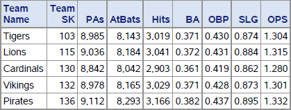
Output 8.14 byMonth Splits

Output 8.15 byDayOfWeek Splits

Output 8.16 byPlayerMonth Splits

And, we pointed out to the IT users, this approach could also perhaps use the SAS macro language.
8.3.1 Using Parameter Files to Define Aggregates
The approach of hard-coding to define and calculate the splits can become unwieldy fairly quickly, and our business users have asked if there is a way to make this easier. They have said that there are likely cases where there are dozens of possible splits and they would like to be able to add new splits without having to add new code.
We, of course, expected that question and were prepared to demonstrate how we could use data sets (also known as parameter files) to define and calculate the same splits as presented in the previous section. The first step is to create a parameter file that defines the splits. A screenshot of a simple example of such a parameter file is shown below. For the purposes of this Proof of Concept, we decided to keep this parameter file simple. For example, we are assuming that any field that is part of the key is also included in the data portion. The data set Chapter8Parmfile in the TEMPLATE library includes the definitions for all the splits included in the previous example.
Output 8.17 First 12 Rows of Chapter8Parmfile

The use of the macro language to generate the code to define hash table objects from metadata (i.e., a parameter file) was introduced in the Chapter 7 section, “Using a Macro to Create the Hash Object Method Calls.” We will use a similar macro here. Since the next chapter will introduce what we believe is a more flexible approach that will better meet our users’ needs, we decided not to try to generalize the macro logic to handle the requirements addressed in Chapter 7 as well as what we need to do here. Given the metadata approach, the code for each hash table is the same. We just need to use an appropriate WHERE clause for each set of hash object method calls.
In order to impress upon the IT users the fact that SAS has a very broad range of tools, we decided to use the macro language, a PROC SQL step, and a DATA step for this example. Let us cover each of these individually.
Program 8.15 - Chapter 8 Multiple Splits Parameterized.sas (Part 1)
%macro createHash ❶
(hashTable = hashTable
,parmfile = template.Chapter8ParmFile
);
lr = 0;
dcl hash &hashTable(ORDERED:"A"); ❷
do while(lr=0);
set &parmfile end=lr; ❸
where upcase(hashTable) = "%upcase(&hashTable)";
if Is_A_key then &hashTable..DefineKey(Column); ❹
&hashTable..DefineData(Column); ❺
end;
&hashTable..DefineDone(); ❻
%mend createHash;
❶ Define the macro with two parameters: the name of the variable that provides the name for the hash object to be created; and the name of the data set that contains the metadata which defines each hash object.
❷ Declare the hash table. The ORDERED:"A" argument tag is used since we want the items in the table to be logically ordered by the key so the output data set is sorted by the key.
❸ Loop through the schema metadata, reading only the definition data for the specified hash table.
❹ If the current column is a key, use the DEFINEKEY method to specify that the column is to be used in the key portion.
❺ Use the DEFINEDATA method to specify that the column is to be used in the data portion. Note that this macro makes the assumption that columns in the key portion should also be included in the data portion.
❻ Use the DEFINEDONE method to finalize the creation of the hash object instance.
By using this macro we can create each hash object table with a single macro call. However, we still need a separate macro call for each hash table. We could certainly write different or additional macro code to loop through all the desired hash tables. Since our users and the developers are not fully familiar with the range of available SAS tools, we decided to take a different approach to handle this looping.
There are actually three sets of repetitive code. We need to generate code to perform the following functions for each split (i.e., hash table):
● Define the hash tables using the createHash macro.
● The statements to invoke the linked section to perform the calculation for each hash table.
● The method calls to create output data sets corresponding to the contents of each hash table.
The following PROC SQL statements create macro variables for each of these three repetitive blocks of code.
Program 8.15 - Chapter 8 Multiple Splits Parameterized.sas (Part 2)
proc sql noprint; ❶
select distinct cats('%createHash(hashTable='
,hashTable
,")"
)
into:createHashCalls separated by " "
from template.Chapter8ParmFile; ❷
select distinct cats("h_pointer="
,hashTable
,";"
,"link slashline"
) ❸
into:calcHash separated by ";"
from template.Chapter8ParmFile;
select distinct cats(hashTable
,'.output(dataset:"_'
,hashTable
,'(drop=_:)")'
) ❹
into:outputHash separated by ";"
from template.Chapter8ParmFile;
quit;
❶ Use the SQL procedure to create the needed macro variables. The NOPRINT option is used as we don’t need to see the output listing of the individual selected rows.
❷ Use the CATS function to concatenate the needed text strings, with the value of the hashTable variable from the metadata parameter file template.Chapter8ParmFile. The DISTINCT option ensures that each distinct value of the hashTable variable is included only once and the SEPARATED BY clause ensures that each generated value is included in the macro variable createHashCalls. Since macro calls do not need a semicolon we used a space as the separator character. For consistency with the next two macro variables, we chose to use a semicolon (;) here as well.
❸ A comparable CATS function call is used to create the statements to assign the hashTable object identifier to our reusable object type variable and to use the LINK statement to perform the needed calculations.
❹ A comparable CATS function call is used to create the statements that output the resulting data sets from each hash table object.
Output 8.18 Listing of Created Macro Variable Names and Values

The DATA step that does the splits calculations is virtually the same as the program discussed in the previous section. The only difference is the repetitive code has been replaced by macro variable references.
Program 8.15 - Chapter 8 Multiple Splits Parameterized.sas (Part 3)
data _null_;
/* define the lookup hash object tables */
dcl hash players(dataset:"dw.players(rename=(Player_ID=Batter_ID))"
,multidata:"Y");
players.defineKey("Batter_ID");
players.defineData("Batter_ID","Team_SK","Last_Name","First_Name"
,"Start_Date","End_Date");
players.defineDone();
dcl hash teams(dataset:"dw.teams");
teams.defineKey("Team_SK");
teams.defineData("Team_Name");
teams.defineDone();
dcl hash games(dataset:"dw.games");
games.defineKey("Game_SK");
games.defineData("Date","Month","DayOfWeek");
games.defineDone();
/* define the result hash object tables */
dcl hash h_pointer;
&createHashCalls ❶
if 0 then set dw.players(rename=(Player_ID=Batter_ID))
dw.teams
dw.games;
format PAs AtBats Hits comma6. BA OBP SLG OPS 5.3;
lr = 0;
do until(lr);
set dw.AtBats end = lr;
call missing(Team_SK,Last_Name,First_Name,Team_Name,Date,Month,DayOfWeek);
games.find();
players_rc = players.find();
do while(players_rc = 0);
if (Start_Date le Date le End_Date) then leave;
players_rc = players.find_next();
end;
if players_rc ne 0
then call missing(Team_SK,First_Name,Last_Name);
teams.find();
&calcHash; ❷
end;
&outputHash; ❸
stop;
slashline:
call missing(PAs,AtBats,Hits,_Bases,_Reached_Base);
rc = h_pointer.find();
PAs + 1;
AtBats + Is_An_AB;
Hits + Is_A_Hit;
_Bases + Bases;
_Reached_Base + Is_An_OnBase;
BA = divide(Hits,AtBats);
OBP = divide(_Reached_Base,PAs);
SLG = divide(_Bases,AtBats);
OPS = sum(OBP,SLG);
h_pointer.replace();
return;
run;
❶ Replace the (in this case) five macro calls with a reference to the macro variable whose value is the five macro calls.
❷ Replace the five sets of assignment and LINK statements with a reference to the macro variable whose value is the five sets of statements.
❸ Replace the five sets OUTPUT method calls with a reference to the macro variable whose value is the five method calls.
Running this program creates exactly the same output as seen above in Output 8.12-8.16. The approach of parameterizing (via metadata) the list of splits to be calculated has the important additional benefit that additional splits can be defined and calculated without having to change the code. All that is needed is to update the metadata table to define additional splits. When we present that to our users we will suggest that a web-based interface could be built (again, using SAS software) to maintain and update a flexible metadata structure to support defining such splits.
8.4 Summary
The reaction to these sample programs was very positive and both the business and IT users were interested in the next phase of our Proof of Concept. In Chapter 9 we will further generalize and parameterize the samples presented in this chapter. We will also leverage the sample presented in this chapter in our case studies in Chapters 12 and 13.