It is common to accuse systems, particularly AI systems or systems incorporating AI, of being ‘biased’ or ‘unfair’. These two words are often used synonymously, but we will follow the International Organization for Standardization (ISO) paradigm and distinguish between them – ‘bias’ being a statistical phenomenon, capable of precise definition, and ‘fairness’ an ethics one, whose interpretation depends on, for example, ‘established norms’, and hence perceptions of fairness can vary. More precisely, we adopt the following based on work under way in ISO/IEC SC 42, one of the standards development organisations examining the issue:

‘Bias’ is a systematic difference in treatment of certain objects, people, or groups in comparison to others (ISO/IEC, 2021a, Definition 3.2.2; ISO/IEC, 2021b).

‘Fairness’ is treatment, behaviour, or outcomes that respect established facts, beliefs, and norms and are not determined or affected by favouritism or unjust discrimination (ISO/IEC, 2022).

This is an important distinction, often lost in the noise of marketing and politics. For example, Facebook have a tool called ‘Fairness Flow’, trumpeted as ‘How we’re using Fairness Flow to help build AI that works better for everyone’ (Kloumann and Tanner, 2021). However, the technical description is much more modest (or ‘realistic’ if one prefers):

Fairness Flow is a technical toolkit that enables our teams to analyze how some types of AI models and labels perform across different groups. Fairness Flow is a diagnostic tool, so it cannot resolve fairness concerns on its own — that would require input from ethicists and other stakeholders, as well as context-specific research. However, Fairness Flow can provide necessary insight to help us understand how some systems in our products perform across user groups (Kloumann and Tanner, 2021).

There is an interesting contrast here: this message mentions stakeholders, but then asks about performance across user groups, not wider stakeholders: see the section ‘Targeted advertising is biased’ later in this chapter. In fact, neither are really a correct description. If we ask Fairness Flow about gender bias in automated hiring tools, we are probably interested, not in gender bias with respect to the user (the human resources operative), but with respect to the data subject (the person being considered for hiring).

In this chapter we will look at some of the basic statistics underpinning the definition of bias, and some examples of bias, both intended and unintended, in everyday life. One example will be gender-biased car insurance pricing, where the raw data show a bias (men have more, and worse, accidents), and then the question is whether taking this difference into account in pricing is fair.

CONSEQUENCES OF THE BIAS DEFINITION

There are various consequences of measuring performance across user groups:

In practice we also need the sets, and the amount of bias, to be large enough that the amount of bias is unlikely to have arisen by chance. Let us suppose we have populations consisting of equal numbers of A and B, and that we have a picking system that does not differentiate between members of A and members of B (that it is unbiased between A and B). A statistician would say that we have the null hypothesis, that there is no difference between A and B as far as this system is concerned. Let us take a look at the probability of our system picking different numbers of members from different population sizes:

• Picking two members out of a population of four. Here the chance of picking the two A members is one-sixth (because the chance of picking an A the first time is one-half, and there are then one A and two B left, so the chance of picking a second A is one-third). The same for two B members and picking one of each class (AB or BA) has a probability of two-thirds.
• Picking three members out of a population of six. Here the chance of AAA is one-twentieth, as is BBB, and AAB and ABB each have chance nine-twentieths.
• Picking four members out of a population of eight. Here the chance of AAAA (or BBBB) is one-seventieth, AAAB (or BBBA) is eight-thirty-fifths and AABB is eighteen-thirty-fifths.
• Picking five members out of a population of ten. Here the chance of AAAAA (or BBBBB) is 1 in 252; AAAAB (or BBBBA) is 25 in 252, and AAABB (or BBBAA) is 100 in 252.
• Picking 10 members out of a population of 20. The probabilities are now 1/184,756 ≈ 0.0000054, 25/46,189 ≈ 0.00054, 2,025/184,756 ≈ 0.011, 3,600/46,189 ≈ 0.078, 11,025/46,189 ≈ 0.24, 15,876/46,189 ≈ 0.34 for an even split, and then the same in reverse.
• Picking 50 members out of a population of 100. Here the chance of an exactly even split is roughly 5 per cent, and all other probabilities are less, so we cannot even expect an unbiased system to give us a perfectly unbiased answer.

Statisticians are used to this problem, and approach it by asking not what the probability of an exact value is, but what the probability of seeing at least (or at most) this value is. More formally, suppose T is the value we are observing (in our case the number of A chosen). Then we ask, for a threshold value t, ‘what is the probability that T > t under the null hypothesis’ (assuming that we are interested in the question ‘are too many A being chosen?’). If we are observing an event t such that this probability is very small, then we can conclude:

Either: the null hypothesis is false (in our case the picking system is differentiating between A and B).

Or: we have observed an unlikely event.

A statistician chooses some significance level α, observes t, calculates the probability p that T > t under the null hypothesis (what is the probability that I would have seen something at least this surprising?) and compares p with α. If p is smaller, then the usual jargon is that the statistician ‘rejects the null hypothesis’ but note that this does not mean the null hypothesis is false, as we could always have observed an unlikely event.

This brings us to the key question: what should α be? A common value in science is α = 0.05, but this should be associated with the conclusion ‘further experiments are required’: one-twentieth isn’t that improbable. Other common values are 0.01 or 0.001, but much smaller values are also used. For example, the Higgs boson discovery (CMS Collaboration, 2012) was announced with α = 1/3,500,000 (this value is 5σ from statistical theory) and the accepted standard in genome analysis (G. M. Clarke et al., 2011) is 5 × 10–8 (1 in 20 million).

There are two warning notes that should be sounded.

We have been talking about a single direction of bias (choosing A over B). However, there can be many possible directions, and they may not be binary. For example, the UK’s Equality Act 2010 defines nine protected characteristics, and while a few are binary, many, such as age, are not. Even if they were all binary, and if our system were unbiased, while the chance of failing a given one of them at the α = 0.05 is, by definition, one-twentieth, the chance of failing one of nine at that level is 37 per cent. Hence, it is quite likely that a simplistic test will declare that a system that is in fact unbiased is biased according to one of these characteristics. That is, if we perform the experiments first then choose the characteristic. A simple solution to this is known as the Bonferroni–Dunn correction (Bonferroni, 1936; Dunn, 1961) and replaces α by α*= α/n if we have n different directions of bias. A slightly more subtle correction is the Šidak correction (Šidak, 1968), with α* = 1 – (1 – α)^1/n, but the difference is very small in practice, and a statistician should probably be consulted if the difference matters. Hence we should be looking at α* being 0.0056 (or 0.0057 if using the Šidak version) for each of nine directions of bias, if we are to have a 0.05 chance of declaring an unbiased system to be possibly biased.

These are tests for statistical significance, not practical significance. The distinction is especially important in medicine, where the phrase ‘clinical significance’ is used to indicate that the effect actually matters.

BIAS IN EVERYDAY LIFE

Life as we encounter it is actually full of biases: some explicit and some implicit, some human-constructed and some not. An example of a human-constructed explicit sex bias was the male-preference primogeniture rule (until 2015) that the eldest male child inherited the throne of the UK, with a female child only inheriting if there were no male children. Historically there were very many such explicit human-created sex biases, and while many have been legally abolished, their effects linger. To continue the example, male-preference primogeniture means that choosing a random monarch of the UK is much more likely (thirteen-sixteenths, excluding ‘William and Mary’) to choose a king than a queen.

Another bias, seemingly created by nature, is that women tend to live longer than men. This is true even if we set aside issues such as war, which tend to kill young men. Life expectancy at 65 in the UK shows that women can expect to live two years longer than men, on average (Institute and Faculty of Actuaries, 2018). For centuries, insurance companies and annuity providers have dealt with this by quoting different rates for men and women, with the intention of unbiasing the expected payout. However, this approach has been ruled illegal in the European Union (‘Test-Achats Ruling’) (European Court of Justice, 2011) and all insurance rates must be quoted without bias for gender. This means that the rates are unbiased, but the payouts are now biased – a woman can expect to receive more than a man. This is an example of a general principle: where there is a bias due to nature, we cannot remove it, only change where it shows up.

In many societies, but certainly in the UK, men, particularly young men, have more, and worse, road traffic accidents than women. The Guardian newspaper (2004) notes that men are guilty of causing 94 per cent of the accidents involving death or bodily harm. Hence insurance companies used to quote higher premiums for male drivers. Again, this is now illegal in the European Union. However, other factors, such as car type and driver’s occupation, can be used. This was studied in the context of the UK car insurance market by McDonald (2015). He observed that the ruling was effective in eliminating direct gender discrimination. However, in the UK, many occupations have a strong gender bias – among his examples were plasterer (96 per cent male) and dental nurse (100 per cent female). Indeed, he found dental nurses were being charged 9 per cent less than the average for car insurance, and plasterers 9 per cent more.

The conclusions of McDonald require careful interpretation.

It is found that the Ruling has been effective at stopping direct discrimination by gender. However, for young drivers, for whom the difference in risk between males and females is greatest, there is evidence that firms are engaging in indirect discrimination using occupations as a proxy for gender, with insurance prices becoming relatively lower (higher) for those in female (male) dominated jobs. The implications of this go beyond the motor insurance market as it is possible that this could also be observed in other markets affected by the Ruling, for example pension annuities.

The last sentence is certainly true and has significant implications. In reading the earlier sentences, we must be careful not to anthropomorphise. These prices come out of a comparison website that is interrogating the pricing engines of the various insurance companies. No human being is engaged in the detailed pricing decisions: they are reached on the basis of a large amount of data analysis. Indeed, these analysis programs may well not have been changed (the author has been informed that in at least one case they were not), just the variables being input had ‘gender’ removed. A common phrase would be ‘occupation is a proxy for gender’, but again this is anthropomorphic: what is happening is that the statistical engines are simply computing correlations, or one might say ‘following the data’.

Differential pricing is intrinsically biased

The car insurance example above illustrates a general fact that many people try to ignore: all differential pricing is biased; and it is biased against those who are charged more. The question is not whether it is biased, the question is whether the bias is acceptable, socially or legally. Gender-biased car insurance was socially acceptable for many years in the EU (and indeed probably still is, despite not being legally acceptable) and is both socially and legally acceptable in many parts of the world today.

An example of differential pricing is train fares. In the UK we are used to paying very different prices depending on whether we are travelling ‘off-peak’:¹ for example, a return from Bath Spa to London varies (at the time of writing) from £214.20 (‘peak’), via £86.80 (‘off-peak’), to £63.00 (‘super off-peak’). While there are complaints about the absolute amount, and the size of the differential, the existence of the differential is very largely unquestioned. The same is very largely true of airline fares, but these depend on many more variables, and are not as regulated, so the effect is harder to measure.

However, there is much anger when the same principle is applied to holidays and the relationship with school term and holiday dates: The Telegraph newspaper (Spocchia and Morris, 2020) talks about ‘The “daylight” robbery’ of school holiday price increases’, and many other similar articles can be found. In fact, the price differential quoted, ‘nearly three times’, is less than the train fare differential, but the public anger is far greater.

These are all examples of a priori pricing: the customer knows in advance what is being charged and, subject to other constraints such as work commitments or school holidays, can choose to pay less by buying a different service. A classic example of a posteriori pricing, where the service is bought first, and then the price established, is a taxi fare. For a conventional metered taxi, the price is determined as a published function of the a posteriori meter readings (distance travelled and time waiting) and various published parameters, generally time of day and day of week or holiday status. However, for services such as Uber and Lyft, the pricing is more dynamic (akin to airline prices). This was investigated by Pandey and Caliskan (2020), and the results popularised by Lu (2020). They specifically analysed ride-hailing in Chicago, and their

results indicate that fares increase for neighborhoods with a lower percentage of people above 40, a lower percentage of below median house price homes, a lower percentage of individuals with a high-school diploma or less, or a higher percentage of non-white individuals.

The last is a protected characteristic, and discrimination here may be illegal. Looking at their maps for the first three characteristics, it is clear that these three characteristics are quite correlated, as might seem reasonable. We do not have the corresponding map for ethnicity, alas, and it would be interesting to know how correlated this is.

This is not the only instance of racial bias appearing in what one would naively expect to be an unbiased demand pricing algorithm. Angwin et al. (2015) report that the price charged by the Princeton Review for its online SAT tutoring services vary by ZIP code, from (in 2015) $6,600 to $8,400. They discovered that:

Asians are almost twice as likely to be offered a higher price than non-Asians. The gap remains even for Asians in lower income neighbourhoods. Consider a ZIP code in Flushing, a neighbourhood in Queens, New York. Asians make up 70.5 percent of the population in this ZIP code. According to the U.S. Census, the median household income in the ZIP code, $41,884, is lower than most, yet The Princeton Review customers there are quoted the highest price.

The student who originally discovered this price differential has a key point. ‘It’s something that makes a very small impact on one individual’s life but can make a big impact to large groups’ (Angwin et al., 2015). This is an important point: if one ethnic group is disproportionately priced out of educational support, there will be a knock-on effect on educational disparities.

Targeted advertising is biased

This is a blindingly obvious statement when one thinks about it: targeting is biasing by choice. Consider placing advertisements in magazines: a manufacturer of combine harvesters is more likely to advertise in Cereals Weekly than in Interior Decorators Weekly. Few people would object to this, and indeed the readers of Interior Decorators Weekly would probably object to a lot of combine harvester advertisements. However, an advertiser for something else, say jobs as a COVID-19 vaccination site assistant, would be as likely to advertise in one as the other.

However, online advertisement targeting, as practised by Facebook in particular, but also by many others, is different. Rather than being driven by explicit choices, such as subscribing to Cereals Weekly, it is driven by the agency’s (Facebook, etc.) desire for profit, which is generally obtained by people clicking on the advertisement. Hence the agency would be likely to place advertisements for combine harvesters next to stories about cereal prices and so on. However, there are not that many of those, so the agency is likely to put the advertisements in front of readers whose behaviour, as tracked by, say, the Facebook pixel (Newberry, 2019; Venkatadri et al., 2018), indicates that they might be interested in combine harvesters.

If we were merely interested in combine harvester sales, this wouldn’t matter so much. However, one of the things advertised on social media is housing, a subject that is protected from racial discrimination under United States law. There were many issues with social media permitting targeted advertisements, but the major firm involved has agreed to prevent such explicit targeting by the advertisers (ACLU, 2019). However, that is not sufficient to avoid bias, as discovered by Ali et al. (2019). The same mechanism that places combine harvester advertisements in front of people likely to buy them (as perceived by the systems) will also place advertisements for houses to buy (rather than rent) preferentially in front of white people, for example.

Another socially relevant commodity advertised on social media is jobs. This has been investigated by Ali et al. (2019), and more recently by Imana et al. (2021). They point out that, under United States law, ‘ads may be targeted based on qualifications, but not on protected categories’. It is not clear whether it is legal to target based on likely interest: naively one might expect advertisements for combine harvester operators to follow the same principles as combine harvesters, and certainly the magazine advertiser would be more likely to use Cereals Weekly than Interior Decorators Weekly.

Their methodology (Imana et al., 2021) was to place ‘two concurrent ads for similar jobs, but for a pair of companies with different de facto gender distributions of employees’. Their conclusion is especially interesting as it illustrates that bias by gender need not be inherent in these processes.

We confirm skew by gender in ad delivery on Facebook, and show that it cannot be justified by differences in qualifications. We fail to find skew in ad delivery on LinkedIn.

As with Princeton Review pricing, the impact on society is much more significant than the impact on individuals, as we see the perpetuation of gender imbalances.

All of this says that the biases we may be aiming for (e.g. safer drivers) are possibly correlated with biases we are not aiming for (e.g. gender), and we are possibly not allowed to have. In this case, we have a choice between not aiming for the original bias (unlikely in the case of an insurance company), or deliberately correcting for the unwanted consequential bias. However, such corrections may actually be illegal, as discussed for lending in the United States (Hao, 2019), or impossible, as it may be illegal to collect the necessary data (e.g. collecting racial data in France).

In the days of manual CV processing and shortlisting, it was common for personnel departments (as ‘human resources’ was then called) to have a separate sheet with demographic data, with the statement that these would not go to the short-listing panel, but only be used for bias monitoring. This mechanism is obsolete, and it is not clear that people would have the same faith in a fully automated process as they used to have in the paper processing. However, the spirit needs to be remembered, and unwanted bias needs to be checked for, rather than just assumed not to exist.

UNINTENDED BIAS

We may be building our AI systems for certain kinds of bias (qualifications, etc.), and we may have corrected for any consequential biases, but other kinds can creep in. There are many causes of this.

Data bias

The data we have may well not be representative of the full range of circumstances in the real world. Indeed, they cannot be completely representative unless the entire world is included in the dataset, so the usual hope is that we have a ‘representative subset’. There are many variants of data bias, currently being enumerated by ISO/IEC with a detailed report: ISO/IEC TR 24027 (ISO/IEC, 2021b). A very important one is sampling bias, which occurs when the dataset sampled is not representative of the demographics or other important features of the real world. As is well-known to pollsters, people chosen at random are not generally representative: it depends on the method of choice, and on the willingness of people to answer questions.

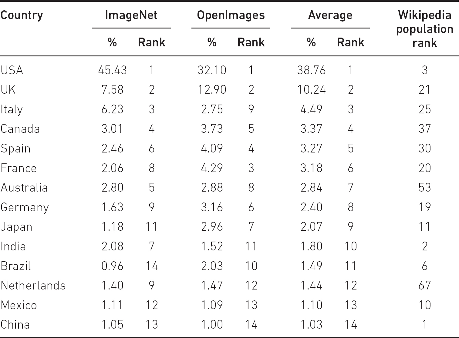
Collecting large amounts of data is extremely expensive, especially if the data need to be labelled. Hence there is a great tendency to rely on ‘well-known’ datasets. Despite being ‘well-known’, these themselves may not be representative: Shankar et al. (2017) report that, for the images they were able to acquire location data for (22 per cent for OpenImages, and a somewhat lower fraction for ImageNet, and with some possibility of error), OpenImages is sourced 32.1 per cent from the United States and 12.9 per cent from the United Kingdom (a total of 45 per cent), and ImageNet is 45.4 per cent from the United States and 7.6 per cent from the United Kingdom (a total of 53 per cent). The top 14 countries, based on average ranking (note that the top 14 countries are identical in the two datasets) are given in Table 3.1, where we have added Wikipedia’s population rank: only 6 of these 14 are in the population rank top 14: conspicuous by their absence are Indonesia and Pakistan (4 and 5 in Wikipedia’s table).

There are many other useful examples in this paper: one study they did looked at the likelihood that images of ‘bridegroom’ would be correctly classified. Not surprisingly (given Table 3.1) images from the USA (and from Australia) were much more likely to be correctly classified than images from Ethiopia or Pakistan. This, and other similar observations, has led to the ‘Datasheets for datasets’ movement (Gebru et al., 2021): ‘By analogy [with electronic component datasheets] we propose that every dataset be accompanied with a datasheet that documents its motivation, composition, collection process, recommended uses, and so on’.

Many other ‘well-known’ data sets contain errors as well, for example the Inside Airbnb dataset (Alsudais, 2021). But the problems with ImageNet are particularly insidious because of the wide use of ImageNet as a starting point. ‘This practice of first training a CNN to perform image classification on ImageNet (i.e. pre-training) and then adapting these features for a new target task (i.e. fine-tuning) has become the de facto standard for solving a wide range of computer vision problems’ (Huh et al., 2016). There is therefore a risk that errors and biases in ImageNet (or other starting points) could persist through the ‘fine-tuning’, even if the fine-tuning data were perfect. That this is not a purely theoretical risk is shown by Steed and Caliskan (2021). They have many findings, but one is this: ‘Both iGPT and SimCLRv2 embeddings [pretrained on ImageNet] also associate white people with tools and black people with weapons in both classical and modernized versions of the Weapon IAT [Implicit Association Test]’.

Table 3.1 Country of origin of images (Source: Shankar et al., 2017)

Historical bias

All data collected are clearly data from the past. How far into the past is generally unknown, and indeed many internet resources are not clearly dated. We saw one example earlier when we looked at the gender of monarchs of the United Kingdom, but there are many others.

This problem of the persistence of the past, and the stereotypes of the past, or indeed the stereotypes of the present, bedevils language processing in particular, as pointed out by Caliskan et al. (2017). Their example is Google’s translating of Turkish (a language with gender-neutral pronouns) into English (a language with gendered pronouns), so that ‘O bir doktor. O bir hemșire’ becomes ‘He is a doctor. She is a nurse’ has been ‘fixed’ to ‘She is a doctor. She is a nurse’ (after a transitional period in which the user got a dialogue about gender-neutral pronouns). However, the trivial (to a human) change to ‘O bir matematikçi. O bir hemşire’ gives ‘He’s a mathematician. She is a nurse’. The same problem can arise with gendered nouns: the Romanian words ‘profesor’ and ‘profesoara’ are translated into English as ‘professor’ and ‘teacher’ respectively. It should be noted that there is no simple solution to these problems: good language translation is a skilled business requiring, at times, large amounts of context.

Labelling bias

Many applications require labelled data, generally labelled by humans, and there can be errors or human bias (see below) introduced in the labelling process. One might hope that errors were small and not systematic, but this needs to be verified rather than assumed. The labelling process may also introduce systematic errors. The ProPublica study referred to on page 19 also pointed out (Angwin et al., 2016) the confusion in US bail software between three concepts:

There are complex sociological and methodological questions here, not least that an offender who has been refused bail is very unlikely to re-offend while locked up. So we cannot measure the ‘false positives’, that is, people who were refused bail, but who would not have been accused of re-offending if bail had been allowed. A simpler example of label confusion is in the account (Perry, 2019) of bicycle counting in San Diego, which was meant to count cyclists, but also counted bicycles hanging on the back of cars.

Data processing bias

The processing of data, and ML typically has a complicated pipeline of data processing, may introduce errors. Real-world data tend to contain gaps, or ‘missing values’ as statisticians tend to refer to them. A trivial example, which the author uncovered many years ago, consisted of coding Male=1, Female=2, Unknown=9, and then taking averages. This led to incorrect statements about the gender mix of the samples, only spotted when there were enough ‘Unknown’ to make the average 2.1, and the researcher sought the author’s help with this ‘bug’. With a complex pipeline, and many actors involved in the data pipeline, more subtle variants of this can slip through.

Human bias

Humans are biased, whether consciously or unconsciously (Gilvoich and Griffin, 2010). These biases may act in the present, or may have acted in the past, to mean that past data, which are what ML algorithms often rely on to predict the future, are biased. This shows up in employment hiring (Bertrand and Mullainathan, 2004; Stokel-Walker, 2021), and indicates that we should be especially careful of these applications.

Accommodation is another area where discrimination may be illegal in many places, and is in Oregon (Serrano, 2022). However, at least some of the discrimination is computing (not specifically AI)-enabled human discrimination, as reported in Edelman et al. (2016). Since an Airbnb host has more information than would normally be available for a hotel booking, they can also be more discriminatory: ‘requests from guests with distinctively African-American names are roughly 16% less likely to be accepted than identical guests with distinctively white names’. Their conclusion is worth noting: ‘On the whole, our analysis suggests a need for caution: while information facilitates transactions, it also facilitates discrimination’.

While many explanations can be given for human bias, such as general bias, group attribution bias, implicit bias, confirmation bias, in-group bias, out-group homogeneity bias, ‘What you see is all there is’ bias and societal bias, the key point is that ‘real-world’ data may well be biased.

SIMPSON’S PARADOX

‘Simpson’s paradox’ is a phenomenon where the trend in separate groups can disappear, or even be reversed, when the groups are combined. Though it had been noted earlier in the history of statistics, this paradox is normally attributed to Simpson (1951), who made a more systematic study of it. A simple example can be seen in Figure 3.1.

Figure 3.1 Simple illustration of Simpson’s paradox

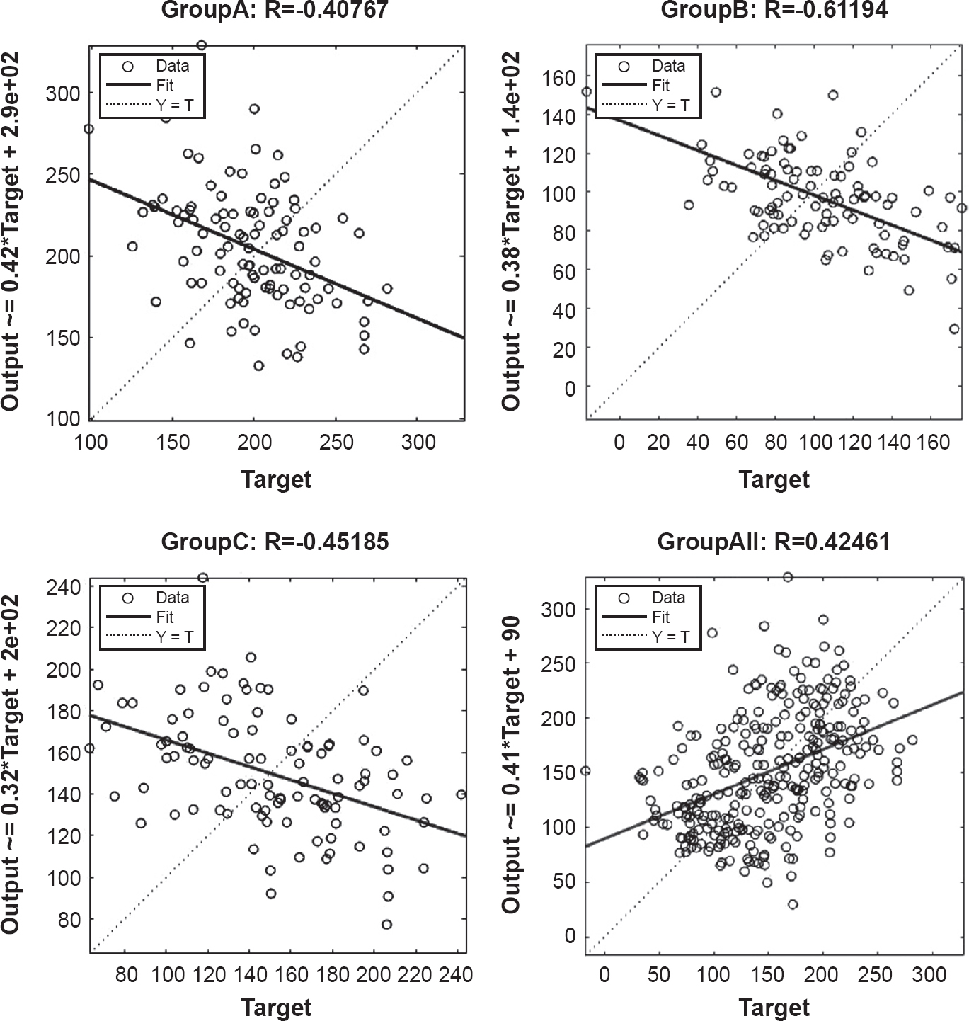
Here we see that in all three Groups, taken individually, the Output is a decreasing function of the Target (with a slope of about –0.4), but across the union of all three groups, it’s an increasing function (with a slope of about +0.4). These data, and more examples, can be found at https://doi.org/10.15125/BATH-01099 (Davenport, in press).

An important example of the paradox is given in Simpson’s paper. Consider first a researcher who is wondering whether the ratio of court to plain cards in a normal (French-suited) pack of 52 cards is different between black and red cards. However, some cards are dirty and some clean, which the researcher also records in case it matters. The researcher records Table 3.2.

Among the dirty cards, 4/7=57 per cent of the court cards are red, but 8/13=61 per cent of the plain cards are red. Hence the dirty plain cards are more likely to be red than the dirty court cards. Among the clean cards, 2/5=40 per cent of the court cards are red, but 12/27=44 per cent of the plain cards are red. Hence, the clean plain cards are more likely to be red than the clean court cards.

But if we ignore the dirty/clean distinction, we get Table 3.3 for a standard (French-suited, 52-card) pack of cards. There is no distinction between red and black: both have 20/26=77 per cent plain.

The apparent conclusion is obvious: we should ignore the clean/dirty distinction.

Now consider Table 3.4.

Among the men, 4/7=57 per cent of the untreated survive, but 8/13=61 per cent of the treated survive. Hence the treated men are more likely to survive. Among the women, 2/5=40 per cent of the untreated survive, but 12/27=44 per cent of the treated survive. Hence the treated women are more likely to survive. Surely the conclusion is that the treatment is good. However, numerically, Table 3.4 is identical to Table 3.2, just with different labels, and if we combine male and female, we will get Table 3.3 again, and observe that there is no difference between treated and untreated, so the treatment might appear valueless. As Simpson says, ‘The treatment can hardly be rejected as valueless when it is beneficial when applied to males and to females.’ An approximate explanation of the paradox in this setting is that we treated a far greater proportion (27/32=84 per cent) of women than men (13/20=65 per cent), but women are more likely to die (18/32=56 per cent) than men (8/20=40 per cent) and we should have done a balanced experiment.

A potentially serious case of Simpson’s paradox in the real world is described by Bickel et al. (1975). They looked at admission to graduate study at the University of California, Berkeley, in fall 1973. Their first analysis looked like Table 3.5.

This shows that, while the overall acceptance rate was 41 per cent, it was 44.3 per cent for men and 34.6 per cent for women, and a statistician would do a χ² test and conclude that the probability of this occurring by chance was vanishingly small. However, at Berkeley, the decision to admit is made by the individual departments, who have widely differing admission ratios and widely differing gender ratios among the applicants. Furthermore, the two are correlated: ‘The proportion of women applicants tends to be high in departments that are hard to get into and low in those that are easy to get into.’ In fact, a more detailed analysis shows that there is a bias in favour of women admitted. As the authors conclude: ‘The bias in the aggregated data stems not from any pattern of discrimination on the part of admissions committees, which seem quite fair on the whole, but apparently from prior screening at earlier levels of the educational system.’

SUMMARY

The first conclusion is that bias-free AI is pointless: we want AI to treat some groups differently from others, that is, to be biased in favour of those groups, since there is no point in using it unless it makes distinctions. However, we want it to make the right distinctions, and there may well be ethical or legal requirements that AI does not have certain biases (e.g. gender, ethnicity, ability). This may actually be a very difficult, or impossible, job: in the case of young drivers it is impossible to be fully biased against accident-prone individuals without being gender-biased in many cultures. However, we can make some comments we hope will be helpful:

1 But not in many countries. A similar trip (Heidelberg to Frankfurt) in Germany varies from €17.90 to €28.90 but depending on the type of train rather than the time of day, and indeed the €17.90 trains seem to be the fastest.