
Computational geometry is a field of mathematics that seeks the development of efficient algorithms to solve problems described in terms of basic geometrical objects. We differentiate between combinatorial computational geometry and numerical computational geometry.
Combinatorial computational geometry deals with the interaction of basic geometrical objects—points, segments, lines, polygons, and polyhedra. In this setting, we have three categories of problems:
- Static problems: The construction of a known target object is required from a set of input geometric objects
- Geometric query problems: Given a set of known objects (the search space) and a sought property (the query), these problems deal with the search of objects that satisfy the query
- Dynamic problems: This is similar to the problems from the previous two categories, with the added challenge that the input is not known in advance, and objects are inserted or deleted between queries/constructions
Numerical computational geometry deals mostly with the representation of objects in space described by means of curves, surfaces, and regions in space bounded by these.
Before we proceed to the development and analysis of the different algorithms in those two settings, it pays to explore the basic background—Plane geometry.
The geometry module of the SymPy library covers basic geometry capabilities. Rather than giving an academic description of all objects and properties in that module, we discover the most useful ones through a series of small self-explanatory Python sessions.
We start with the concepts of point and segment. The aim is to illustrate how easily we can check for collinearity, compute lengths, midpoints, or slopes of segments, for example. We also show how to quickly compute the angle between two segments, as well as decide whether a given point belongs to a segment or not. The following diagram illustrates an example, which we will follow up with the code:

In [1]: from sympy.geometry import Point, Segment, Line,
   ...:                            Circle, Triangle, Curve
In [2]: P1 = Point(0, 0);
   ...: P2 = Point(3, 4);
   ...: P3 = Point(2, -1);
   ...: P4 = Point(-1, 5)
In [3]: statement = Point.is_collinear(P1, P2, P3);
   ...: print "Are P1, P2, P3 collinear?," statement
Are P1, P2, P3 collinear? False
In [4]: S1 = Segment(P1, P2);
   ...: S2 = Segment(P3, P4)
In [5]: print "Length of S1:", S1.length
Length of S1: 5
In [6]: print "Midpoint of S2:", S2.midpoint
Midpoint of S2: Point(1/2, 2)
In [7]: print "Slope of S1", S1.slope
Slope of S1: 4/3
In [8]: print "Intersection of S1 and S2:", S1.intersection(S2)
Intersection of S1 and S2: [Point(9/10, 6/5)]
In [9]: print "Angle between S1, S2:", Segment.angle_between(S1, S2)
Angle between S1, S2: acos(-sqrt(5)/5)
In [10]: print "Does S1 contain P3?", S1.contains(P3)
Does S1 contain P3? False
The next logical geometrical concept is the line. We can perform more interesting operations with lines, and to that effect, we have a few more constructors. We can find their equations; compute the distance between a point and a line, and many other operations:

In [11]: L1 = Line(P1, P2)
In [12]: L2 = L1.perpendicular_line(P3) #perpendicular line to L1
In [13]: print "Parametric equation of L2:", L2.arbitrary_point()
Parametric equation of L2: Point(4*t + 2, -3*t – 1)
In [14]: print "Algebraic equation of L2:", L2.equation()
Algebraic equation of L2: 3*x + 4*y - 2
In [15]: print "Does L2 contain P4?", L2.contains(P4)
Does L2 contain P4? False
In [16]: print "Distance from P4 to L2:", L2.distance(P4)
Distance from P4 to L2: 3
In [17]: print "Is L2 parallel with S2?", L1.is_parallel(S2)
Is L2 parallel with S2? False
The next geometrical concept we are to explore is the circle. We can define a circle by its center and radius, or by three points on it. We can easily compute all of its properties, as shown in the following diagram:
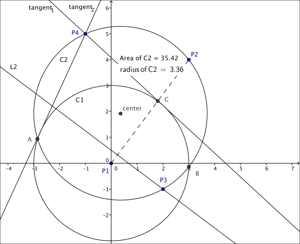
In [18]: C1 = Circle(P1, 3);
   ....: C2 = Circle(P2, P3, P4)
In [19]: print "Area of C2:", C2.area
Area of C2: 1105*pi/98
In [20]: print "Radius of C2:", C2.radius
Radius of C2: sqrt(2210)/14
In [21]: print "Algebraic equation of C2:", C2.equation()
Algebraic equation of C2: (x - 5/14)**2 + (y - 27/14)**2 - 1105/98
In [22]: print "Center of C2:", C2.center
Center of C2: Point(5/14, 27/14)
In [23]: print "Circumference of C2:", C2.circumference
Circumference of C2: sqrt(2210)*pi/7
Computing intersections with other objects, checking whether a line is tangent to a circle, or finding the tangent lines through a exterior point, are simple tasks too:
In [24]: print "Intersection of C1 and C2:
", C2.intersection(C1)
Intersection of C1 and C2:
[Point(55/754 + 27*sqrt(6665)/754, -5*sqrt(6665)/754 + 297/754),
 Point(-27*sqrt(6665)/754 + 55/754, 297/754 + 5*sqrt(6665)/754)]
In [25]: print "Intersection of S1 and C2:
", C2.intersection(S1)
Intersection of S1 and C2:
[Point(3, 4)]
In [26]: print "Is L2 tangent to C2?", C2.is_tangent(L2)
Is L2 tangent to C2? False
In [27]: print "Tangent lines to C1 through P4:
",
                C1.tangent_lines(P4)
Tangent lines to C1 through P4:
[Line(Point(-1, 5),
      Point(-9/26 + 15*sqrt(17)/26, 3*sqrt(17)/26 + 45/26)),
 Line(Point(-1, 5),
      Point(-15*sqrt(17)/26 - 9/26, -3*sqrt(17)/26 + 45/26))]
The triangle is a very useful basic geometric concept. Reliable manipulation of these objects is at the core of computational geometry. We need robust and fast algorithms to manipulate and extract information from them. Let's first show the definition of one, together with a series of queries to describe its properties:
In [28]: T = Triangle(P1, P2, P3)
In [29]: print "Signed area of T:", T.area
Signed area of T: -11/2
In [30]: print "Angles of T:
", T.angles
Angles of T:
{Point(3, 4): acos(23*sqrt(26)/130),
 Point(2, -1): acos(3*sqrt(130)/130),
 Point(0, 0): acos(2*sqrt(5)/25)}
In [31]: print "Sides of T:
", T.sides
Sides of T:
[Segment(Point(0, 0), Point(3, 4)),
 Segment(Point(2, -1), Point(3, 4)),
 Segment(Point(0, 0), Point(2, -1))]
In [32]: print "Perimeter of T:", T.perimeter
Perimeter of T: sqrt(5) + 5 + sqrt(26)
In [33]: print "Is T a right triangle?", T.is_right()
Is T a right triangle? False
In [34]: print "Is T equilateral?", T.is_equilateral()
Is T equilateral? False
In [35]: print "Is T scalene?", T.is_scalene()
Is T scalene? True
In [36]: print "Is T isosceles?", T.is_isosceles()
Is T isosceles? False
Next, note how easily we can obtain representation of the different segments, centers, and circles associated with triangles, as well as the medial triangle (the triangle with vertices at the midpoints of the segments):
In [37]: T.altitudes
Out[37]:
{Point(0, 0) : Segment(Point(0, 0), Point(55/26, -11/26)),
 Point(2, -1): Segment(Point(6/25, 8/25), Point(2, -1)),
 Point(3, 4) : Segment(Point(4/5, -2/5), Point(3, 4))}
In [38]: T.orthocenter     # Intersection of the altitudes
Out[38]:
Point((3*sqrt(5) + 10)/(sqrt(5) + 5 + sqrt(26)), (-5 + 4*sqrt(5))/(sqrt(5) + 5 + sqrt(26)))
In [39]: T.bisectors()    # Angle bisectors
Out[39]:
{Point(0, 0) : Segment(Point(0, 0), Point(sqrt(5)/4 + 7/4, -9/4 + 5*sqrt(5)/4)),
 Point(2, -1): Segment(Point(3*sqrt(5)/(sqrt(5) + sqrt(26)),  4*sqrt(5)/(sqrt(5) + sqrt(26))),
           Point(2, -1)),
 Point(3, 4) : Segment(Point(-50 + 10*sqrt(26), -5*sqrt(26) + 25), Point(3, 4))}
In [40]: T.incenter     # Intersection of angle bisectors
Out[40]:
Point((3*sqrt(5) + 10)/(sqrt(5) + 5 + sqrt(26)), (-5 + 4*sqrt(5))/(sqrt(5) + 5 + sqrt(26)))
In [41]: T.incircle
Out[41]:
Circle(Point((3*sqrt(5) + 10)/(sqrt(5) + 5 + sqrt(26)),
             (-5 + 4*sqrt(5))/(sqrt(5) + 5 + sqrt(26))),
       -11/(sqrt(5) + 5 + sqrt(26)))
In [42]: T.inradius
Out[42]: -11/(sqrt(5) + 5 + sqrt(26))
In [43]: T.medians
Out[43]:
{Point(0, 0) : Segment(Point(0, 0), Point(5/2, 3/2)),
 Point(2, -1): Segment(Point(3/2, 2), Point(2, -1)),
 Point(3, 4) : Segment(Point(1, -1/2), Point(3, 4))}
In [44]: T.centroid     # Intersection of the medians
Out[44]: Point(5/3, 1)
In [45]: T.circumcenter   # Intersection of perpendicular bisectors
Out[45]: Point(45/22, 35/22)
In [46]: T.circumcircle
Out[46]: Circle(Point(45/22, 35/22), 5*sqrt(130)/22)
In [47]: T.circumradius
Out[47]: 5*sqrt(130)/22
In [48]: T.medial
Out[48]: Triangle(Point(3/2, 2), Point(5/2, 3/2), Point(1, -1/2))
Here are some other interesting operations with triangles:
- Intersection with other objects
- Computation of the minimum distance from a point to each of the segments
- Checking whether two triangles are similar
In [49]: T.intersection(C1)
Out[49]: [Point(9/5, 12/5), Point(sqrt(113)/26 + 55/26, -11/26 + 5*sqrt(113)/26)]
In [50]: T.distance(T.circumcenter)
Out[50]: sqrt(26)/11
In [51]: T.is_similar(Triangle(P1, P2, P4))
Out[51]: False
The other basic geometrical objects currently coded in the geometry module are:
LinearEntity: This is a superclass with three subclasses:Segment,Line, andRay. The classLinearEntityenjoys the following basic methods:are_concurrent(o1, o2, ..., on)are_parallel(o1, o2)are_perpendicular(o1, o2)parallel_line(self, Point)perpendicular_line(self, Point)perpendicular_segment(self, Point)
Ellipse: This is an object with a center, together with horizontal and vertical radii.Circleis, as a matter of fact, a subclass ofEllipsewith both radii equal.Polygon: This is a superclass that we can instantiate by listing a set of vertices.Trianglesare a subclass ofPolygon, for example. The basic methods of Polygon are:areaperimetercentroidsidesvertices
RegularPolygon. This is a subclass ofPolygon, with extra attributes:apothemcentercircumcircleexterior_angleincircleinterior_angleradiusTip
For more information about this module, refer to the official SymPy documentation at http://docs.sympy.org/latest/modules/geometry/index.html.
There is also a nonbasic geometric object—a curve, which we define by providing parametric equations, together with the interval of definition of the parameter. It currently does not have many useful methods, other than those describing its constructors. Let's illustrate how to deal with these objects. For example, a three-quarters arc of an ellipse could be coded as follows:
In [52]: from sympy import var, pi, sin, cos
In [53]: var('t', real=True)
In [54]: Arc = Curve((3*cos(t), 4*sin(t)), (t, 0, 3*pi/4))
To end the exposition on basic objects from the geometry module in the SymPy library, we must mention that we can apply any basic affine transformations to any of the previous objects. This is done by combination of the methods reflect, rotate, translate, and scale:
In [55]: T.reflect(L1)
Out[55]: Triangle(Point(0, 0), Point(3, 4), Point(-38/25, 41/25))
In [56]: T.rotate(pi/2, P2)
Out[56]: Triangle(Point(7, 1), Point(3, 4), Point(8, 3))
In [57]: T.translate(5,4)
Out[57]: Triangle(Point(5, 4), Point(8, 8), Point(7, 3))
In [58]: T.scale(9)
Out[58]: Triangle(Point(0, 0), Point(27, 4), Point(18, -1))
In [59]: Arc.rotate(pi/2, P3).translate(pi,pi).scale(0.5)
Out[59]:
Curve((-2.0*sin(t) + 0.5 + 0.5*pi, 3*cos(t) - 3 + pi), (t, 0, 3*pi/4))
With these basic definitions and operations, we are ready to address more complex situations. Let's explore these new challenges next.