We may create matrices from data as ndarray instances in three different ways: manually from standard input, by assigning to each entry a value from a function, or by retrieving the data from external files.

Let us create some example matrices to illustrate some of the functions defined in the previous table. As before, we start an iPython session:

In [1]: import numpy as np, matplotlib.pyplot as plt, 
   ...: scipy.linalg as spla, scipy.sparse as spsp, 
   ...: scipy.sparse.linalg as spspla
In [2]: A = np.array([[1,2],[4,16]]); ...: A
Out[2]:
array([[ 1,  2],
       [ 4, 16]])
In [3]: B = np.fromfunction(lambda i,j: (i-1)*(j+1),
   ...:                     (3,2), dtype=int); 
   ...: print B
   ...:
 [[-1 -2]
  [ 0  0]
  [ 1  2]]
In [4]: np.diag((1j,4))
Out[4]:
array([[ 0.+1.j,  0.+0.j],
       [ 0.+0.j,  4.+0.j]])

Special matrices with predetermined zeros and ones can be constructed with the following functions:

In [5]: np.empty_like(A)
Out[5]:
array([[140567774850560, 140567774850560],
       [     4411734640, 562954363882576]])

Of notable importance are arrays constructed as numerical ranges.

Special matrices with numerous applications in linear algebra can be easily called from within NumPy and the module scipy.linalg.

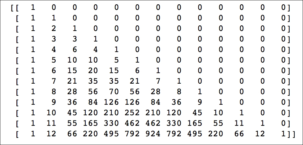
For instance, one fast way to obtain all binomial coefficients of orders up to a large number (the corresponding Pascal triangle) is by means of a precise Pascal matrix. The following example shows how to compute these coefficients up to order 13:

In [6]: print spla.pascal(13, kind='lower')

Besides these basic constructors, we can always stack arrays in different ways:

Let us observe some of these constructors in action:

In [7]: np.tile(A, (2,3))   # 2 rows, 3 columns
Out[7]:
array([[ 1,  2,  1,  2,  1,  2],
       [ 4, 16,  4, 16,  4, 16],
       [ 1,  2,  1,  2,  1,  2],
       [ 4, 16,  4, 16,  4, 16]])
In [8]: spla.block_diag(A,B)
Out[8]:
array([[ 1,  2,  0,  0],
       [ 4, 16,  0,  0],
       [ 0,  0, -1, -2],
       [ 0,  0,  0,  0],
       [ 0,  0,  1,  2]])

For the matrix class, the usual way to create a matrix directly is to invoke either numpy.mat or numpy.matrix. Observe how much more comfortable is the syntax of numpy.matrix than that of numpy.array, in the creation of a matrix similar to A. With this syntax, different values separated by commas belong to the same row of the matrix. A semi-colon indicates a change of row. Notice the casting to the matrix class too!

In [9]: C = np.matrix('1,2;4,16'); 
   ...: C
Out[9]:
matrix([[ 1,  2],
        [ 4, 16]])

These two functions also transform any ndarray into matrix. There is a third function that accomplishes this task: numpy.asmatrix:

In [10]: np.asmatrix(A)
Out[10]:
matrix([[ 1,  2],
        [ 4, 16]])

For arrangements of matrices composed by blocks, besides the common stack operations for ndarray described before, we have the extremely convenient function numpy.bmat. Note the similarity with the syntax of numpy.matrix, particularly the use of commas to signify horizontal concatenation and semi-colons to signify vertical concatenation:

In [11]: np.bmat('A;B')        In [12]: np.bmat('A,C;C,A')
Out[11]:                       Out[12]:
matrix([[ 1,  2],              matrix([[ 1,  2,  1,  2],
        [ 4, 16],                      [ 4, 16,  4, 16],
        [-1, -2],                      [ 1,  2,  1,  2],
        [ 0,  0],                      [ 4, 16,  4, 16]])
        [ 1,  2]])

There are seven different ways to input sparse matrices. Each format is designed to make a specific problem or operation more efficient. Let us go over them in detail:

They can be populated in up to five ways, three of which are common to every sparse matrix format:

They all have several different extra input methods, each specific to their storage format.

Let us show by example how to read an interesting matrix in the Rutherford-Boeing matrix exchange format, Pajek/football. This 35 × 35 matrix with 118 non-zero entries can be found in the collection at www.cise.ufl.edu/research/sparse/matrices/Pajek/football.html.

It is an adjacency matrix for a network of all the national football teams that attended the FIFA World Cup celebrated in France in 1998. Each node in the network represents one country (or national football team) and the links show which country exported players to another country.

This is a printout of the football.rb file:

The header of the file (the first four lines) contains important information:

We proceed to opening the file for reading, storing each line after the header in a Python list, and extracting from the relevant lines of the file, the data we require to populate the vectors indptr, indices, and data. We finish by creating the corresponding sparse matrix called football in the CSR format, with the data, indices, pointers method:

In [22]: f = open("football.rb", 'r'); 
   ....: football_list = list(f); 
   ....: f.close()
In [23]: football_data = np.array([])
In [24]: for line in range(4, 4+12):
   ....:     newdata = np.fromstring(football_list[line], sep=" ")
   ....:     football_data = np.append(football_data, newdata)
   ....:
In [25]: indptr = football_data[:35+1] - 1; 
   ....: indices = football_data[35+1:35+1+118] - 1; 
   ....: data = football_data[35+1+118:]
In [26]: football = spsp.csr_matrix((data, indices, indptr),
   ....:                            shape=(35,35))

At this point, it is possible to visualize the network with its associated graph, with the help of a Python module called networkx. We obtain the following diagram depicting as nodes the different countries. Each arrow between the nodes indicates the fact that the originating country has exported players to the receiving country:

One way to accomplish this task is as follows:

In [27]: import networkx
In [28]: G = networkx.DiGraph(football)
In [29]: f = open("football_nodename.txt"); 
   ....: m = list(f); 
   ....: f.close()
In [30]: def rename(x): return m[x]
In [31]: G = networkx.relabel_nodes(G, rename)
In [32]: pos = networkx.spring_layout(G) 
In [33]: networkx.draw_networkx(G, pos, alpha=0.2, node_color='w',
   ....:                        edge_color='b')

The module scipy.sparse borrows from NumPy some interesting concepts to create constructors and special matrices:

Both functions diags and rand deserve examples to show their syntax. We will start with a sparse matrix of size 14 × 14 with two diagonals: the main diagonal contains 1s, and the diagonal below contains 2s. We also create a random matrix with the function scipy.sparse.rand. This matrix has size 5 × 5, with 25 percent non-zero elements (density=0.25), and is crafted in the LIL format:

In [34]: diagonals = [[1]*14, [2]*13]
In [35]: print spsp.diags(diagonals, [0,-1]).todense()
[[ 1.  0.  0.  0.  0.  0.  0.  0.  0.  0.  0.  0.  0.  0.]
 [ 2.  1.  0.  0.  0.  0.  0.  0.  0.  0.  0.  0.  0.  0.]
 [ 0.  2.  1.  0.  0.  0.  0.  0.  0.  0.  0.  0.  0.  0.]
 [ 0.  0.  2.  1.  0.  0.  0.  0.  0.  0.  0.  0.  0.  0.]
 [ 0.  0.  0.  2.  1.  0.  0.  0.  0.  0.  0.  0.  0.  0.]
 [ 0.  0.  0.  0.  2.  1.  0.  0.  0.  0.  0.  0.  0.  0.]
 [ 0.  0.  0.  0.  0.  2.  1.  0.  0.  0.  0.  0.  0.  0.]
 [ 0.  0.  0.  0.  0.  0.  2.  1.  0.  0.  0.  0.  0.  0.]
 [ 0.  0.  0.  0.  0.  0.  0.  2.  1.  0.  0.  0.  0.  0.]
 [ 0.  0.  0.  0.  0.  0.  0.  0.  2.  1.  0.  0.  0.  0.]
 [ 0.  0.  0.  0.  0.  0.  0.  0.  0.  2.  1.  0.  0.  0.]
 [ 0.  0.  0.  0.  0.  0.  0.  0.  0.  0.  2.  1.  0.  0.]
 [ 0.  0.  0.  0.  0.  0.  0.  0.  0.  0.  0.  2.  1.  0.]
 [ 0.  0.  0.  0.  0.  0.  0.  0.  0.  0.  0.  0.  2.  1.]]
In [36]: S_25_lil = spsp.rand(5, 5, density=0.25, format='lil')
In [37]: S_25_lil
Out[37]:
<5x5 sparse matrix of type '<type 'numpy.float64'>'
        with 6 stored elements in LInked List format>
In [38]: print S_25_lil
  (0, 0)    0.186663044982
  (1, 0)    0.127636181284
  (1, 4)    0.918284870518
  (3, 2)    0.458768884701
  (3, 3)    0.533573291684
  (4, 3)    0.908751420065
In [39]: print S_25_lil.todense()
[[ 0.18666304  0.          0.          0.          0.        ]
 [ 0.12763618  0.          0.          0.          0.91828487]
 [ 0.          0.          0.          0.          0.        ]
 [ 0.          0.          0.45876888  0.53357329  0.        ]
 [ 0.          0.          0.          0.90875142  0.        ]]

Similar to the way we combined ndarray instances, we have some clever ways to combine sparse matrices to construct more complex objects:

A linear operator is basically a function that takes as input a column vector and outputs another column vector, by left multiplication of the input with a matrix. Although technically, we could represent these objects just by handling the corresponding matrix, there are better ways to do this.

In the scipy.sparse.linalg module, we have a common interface that handles these objects: the LinearOperator class. This class has only the following two attributes and three methods:

Its usage is best explained through an example. Consider two functions that take vectors of size 3, and output vectors of size 4, by left multiplication with two respective matrices of size 4 × 3. We could very well define these functions with lambda predicates:

In [40]: H1 = np.matrix("1,3,5; 2,4,6; 6,4,2; 5,3,1"); 
   ....: H2 = np.matrix("1,2,3; 1,3,2; 2,1,3; 2,3,1")
In [41]: L1 = lambda x: H1.dot(x); 
   ....: L2 = lambda x: H2.dot(x)
In [42]: print L1(np.ones(3))
[[  9.  12.  12.   9.]]
In [43]: print L2(np.tri(3,3))
 [[ 6.  5.  3.]
  [ 6.  5.  2.]
  [ 6.  4.  3.]
  [ 6.  4.  1.]]

Now, one issue arises when we try to add/subtract these two functions, or multiply any of them by a scalar. Technically, it should be as easy as adding/subtracting the corresponding matrices, or multiplying them by any number, and then performing the required left multiplication again. But that is not the case.

For instance, we would like to write (L1+L2)(v) instead of L1(v) + L2(v). Unfortunately, doing so will raise an error:

TypeError: unsupported operand type(s) for +: 'function' and 
'function'

Instead, we may instantiate the corresponding linear operators and manipulate them at will, as follows:

In [44]: Lo1 = spspla.aslinearoperator(H1); 
   ....: Lo2 = spspla.aslinearoperator(H2)
In [45]: Lo1 - 6 * Lo2
Out[45]: <4x3 _SumLinearOperator with dtype=float64>
In [46]: print Lo1 * np.ones(3)
[  9.  12.  12.  9.]
In [47]: print (Lo1-6*Lo2) * np.tri(3,3)
[[-27. -22. -13.]
 [-24. -20.  -6.]
 [-24. -18. -16.]
 [-27. -20.  -5.]]

Linear operators are a great advantage when the amount of information needed to describe the product with the related matrix is less than the amount of memory needed to store the non-zero elements of the matrix.

For instance, a permutation matrix is a square binary matrix (ones and zeros) that has exactly one entry in each row and each column. Consider a large permutation matrix, say 1024 × 1024, formed by four blocks of size 512 × 512: a zero block followed horizontally by an identity block, on top of an identity block followed horizontally by another zero block. We may store this matrix in three different ways:

In [47]: P_sparse = spsp.diags([[1]*512, [1]*512], [512,-512], 
   ....:                       dtype=int)
In [48]: P_dense = P_sparse.todense()
In [49]: mv = lambda v: np.roll(v, len(v)/2)
In [50]: P_lo = spspla.LinearOperator((1024,1024), matvec=mv, 
   ....:                              matmat=mv, dtype=int)

In the sparse case, P_sparse, we may think of this as the storage of just 1024 integer numbers. In the dense case, P_dense, we are technically storing 1048576 integer values. In the case of the linear operator, it actually looks like we are not storing anything! The function mv that indicates how to perform the multiplications has a much smaller footprint than any of the related matrices. This is also reflected in the time of execution of the multiplications with these objects:

In [51]: %timeit P_sparse * np.ones(1024)
10000 loops, best of 3: 29.7 µs per loop
In [52]: %timeit P_dense.dot(np.ones(1024))
100 loops, best of 3: 6.07 ms per loop
In [53]: %timeit P_lo * np.ones(1024)
10000 loops, best of 3: 25.4 µs per loop