
The aim of this section is the extraction of information from images. We are going to focus on two cases:
- Image structure
- Object recognition
The goal is the representation of the contents of an image using simple structures. We focus on one case alone: image segmentation. We encourage the reader to explore other settings, such as quadtree decompositions.
Segmentation is a method to represent an image by partition into multiple objects (segments); each of them sharing some common property.
In the case of binary images, we can accomplish this by a process of labeling, as we have shown in a previous section. Let's revisit that technique with an artificial image composed by 30 random disks placed on a 64 x 64 canvas:
In [1]: import numpy as np, matplotlib.pyplot as plt
In [2]: from skimage.draw import circle
In [3]: image = np.zeros((64, 64)).astype('bool')
In [4]: for k in range(30):
   ...:     x0, y0 = np.random.randint(64, size=(2))
   ...:     image[circle(x0, y0, 3)] = True
   ...:
In [5]: from scipy.ndimage import label
In [6]: labels, num_features = label(image)
The variable labels can be regarded as another image, where each of the different objects found in the original image have been given a different number. The background of the image is also considered one more object, and received the number 0 as a label. Its visual representation (on the right in the following figure) presents all the objects from the image, each of them with a different color:

For gray-scale or color images, the process of segmentation is more complex. We can often reduce such an image to a binary representation of the relevant areas (by some kind of thresholding operation after treatment with morphology), and then apply a labeling process. But this is not always possible. Take, for example, the coins image skimage.data.coins. In this image, the background shares the same range of intensity as many of the coins in the background. A thresholding operation will result in failure to segment effectively.
We have more advanced options:
- Clustering methods using, as distance between pixels, the difference between their intensities/colors
- Compression-based methods
- Histogram-based methods, where we use the peaks and valleys in the histogram on an image to break it into segments
- Region-growing methods
- Methods based on partial differential equations
- Variational methods
- Graph-partitioning methods
- Watershed methods
From the standpoint of the SciPy stack, we have mainly two options, a combination of tools from scipy.ndimage and a few segmentation routines in the module skimage.segmentation.
Tip
There is also a very robust set of implementations via bindings to the powerful library Insight Segmentation and Registration Toolkit (ITK). For general information on this library, the best resource is its official site http://www.itk.org/.
We use a simplified wrapper build on top of it: The Python distribution of SimpleITK. This package brings most of the functionality of ITK through bindings to Python functions. For documentation, downloads, and installation, go to http://www.simpleitk.org/.
Unfortunately, at the time this book is being written, the installation is very tricky. Successful installations depend heavily on your Python installation, computer system, libraries installed, and more.
Let's see, by example, the usage of some of these techniques on the particularly tricky image skimage.data.coins. For instance, to perform a simple histogram-based segmentation, we could proceed along these lines:
In [8]: from skimage.data import coins;
   ...: from scipy.ndimage import gaussian_filter
In [9]: image = gaussian_filter(coins(), sigma=0.5)
In [10]: plt.hist(image.flatten(), bins=128);
   ....: plt.show()

There seems to be a clear valley around the intensity 80, in between peaks at intensities 35 and 85. There is another valley around the intensity 112, followed by a peak at intensity 123. There is one more valley around intensity 137, followed by a last peak at intensity 160. We use this information to create four segments:
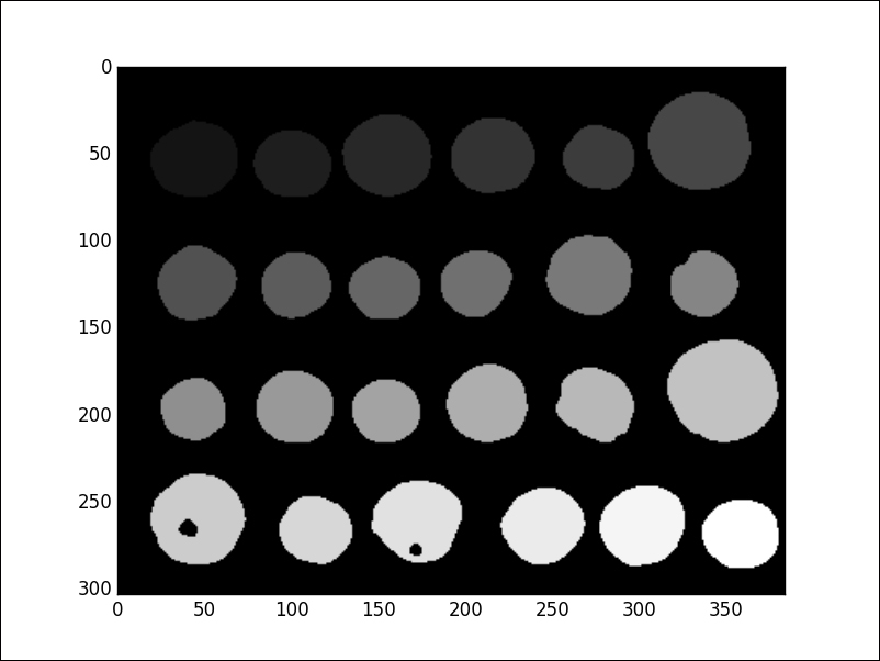
In [11]: level_1 = coins()<=80;
   ....: level_2 = (coins()>80) * (coins()<=112);
   ....: level_3 = (coins()>112) * (coins()<=137);
   ....: level_4 = coins()>137
In [12]: plt.figure();
   ....: plt.subplot2grid((2,4), (0,0), colspan=2, rowspan=2);
   ....: plt.imshow(coins());
   ....: plt.gray();
   ....: plt.subplot2grid((2,4),(0,2));
   ....: plt.imshow(level_1);
   ....: plt.axis('off');
   ....: plt.subplot2grid((2,4),(0,3));
   ....: plt.imshow(level_2);
   ....: plt.axis('off');
   ....: plt.subplot2grid((2,4), (1,2));
   ....: plt.imshow(level_3);
   ....: plt.axis('off');
   ....: plt.subplot2grid((2,4), (1,3));
   ....: plt.imshow(level_4);
   ....: plt.axis('off');
   ....: plt.show()

With a slight modification of the fourth level, we shall obtain a decent segmentation:
In [13]: from scipy.ndimage.morphology import binary_fill_holes
In [14]: level_4 = binary_fill_holes(level_4)
In [15]: labels, num_features = label(level_4)

The result is not optimal. The process has missed a good segmentation of some coins in the fifth column, but mainly in the lowest row.
Improvements can be made if we provide a marker for each of the segments we are interested in obtaining. For instance, we can assume that we know at least one point inside of the locations of those 24 coins. We could then use a watershed transform for that purpose. In the module scipy.ndimage, we have an implementation of this process based on the iterative forest transform:
In [17]: from scipy.ndimage import watershed_ift
In [18]: markers_x = [50, 125, 200, 255];
   ....: markers_y = [50, 100, 150, 225, 285, 350]
In [19]: markers = np.zeros_like(image).astype('int16');
   ....: markers_index = [[x,y] for x in markers_x for y in
   ....:                   markers_y]
In [20]: for index, location in enumerate(markers_index):
   ....:     markers[location[0], location[1]] = index+5
   ....:
In [21]: segments = watershed_ift(image, markers)

Not all coins have been correctly segmented, but those that had been corrected are better defined. To further improve the results of watermarking, we could very well work on the accuracy of the markers or include more than just one point for each desired segment. Note what happens when we add just one more marker per coin, to better segment three of the missing coins:
In [23]: markers[53, 273] = 9;
   ....: markers[130, 212] = 14;
   ....: markers[270, 42] = 23
In [24]: segments = watershed_ift(image, markers)

We can further improve the segmentation by employing, for instance, a graph-partitioning method, like a random walker:
In [26]: from skimage.segmentation import random_walker
In [27]: segments = random_walker(image, markers)

This process correctly breaks the image in to 24 well-differentiated regions, but does not resolve well the background. To take care of this situation, we manually mark, with a-1—those regions we believe are background. We can use the previously calculated masks level_1 and level_2—they clearly represent the image background for these purposes:
In [29]: markers[level_1] = markers[level_2] = -1
In [30]: segments = random_walker(image, markers)
For other segmentation techniques, browse the different routines in the module skimage.segmentation.
Many possibilities arise. Given an image, we might need to collect the location of simple geometric features like edges, corners, linear, circular or elliptical shapes, polygonal shapes, blobs, and so on. We might also need to find more complex objects like faces, numbers, letters, planes, tanks, and so on. Let's examine some examples that we can easily code from within the SciPy stack.
An implementation of Canny's edge detector can be found in the module skimage.feature. This implementation performs a smoothing of the input image, followed by vertical and horizontal Sobel operators, as an aid for the extraction of edges:
In [32]: from skimage.feature import canny
In [33]: edges = canny(coins(), sigma=3.5)

For detection of these basic geometric shapes, we have the aid of the Hough transform. Robust implementations can be found both in the module skimage.transform, and in the imgproc module of OpenCV. Let's examine the usage of the routines in the former by tracking these objects for an artificial binary image. Let's place an ellipse with center (10, 10) and radii 9 and 5 (parallel to the coordinate axes), a circle with center (30, 35) and radius 8, and a line between the points (0, 3) and (64, 40):
In [35]: from skimage.draw import line, ellipse_perimeter,
   ....:                          circle_perimeter
In [36]: image = np.zeros((64, 64)).astype('bool');
   ....: image[ellipse_perimeter(10, 10, 9, 5)] = True;
   ....: image[circle_perimeter(30, 35, 15)] = True;
   ....: image[line(0, 3, 63, 40)] = True
To use the Hough transform for a line, we compute the corresponding H-space (the accumulator), and extract the location of its peaks. In the case of the line version of the Hough transform, the axes of the accumulator represent the angle theta and distance from the origin r in the Hesse normal form of a line r = x cos(θ)+ y sin(θ). The peaks in the accumulator then indicate the presence of the most relevant lines of the given image:
In [37]: from skimage.transform import hough_line, hough_line_peaks
In [38]: Hspace, thetas, distances = hough_line(image);
   ....: hough_line_peaks(Hspace, thetas, distances)
Out[38]:
(array([52], dtype=uint64),
 array([-0.51774851]),
 array([ 3.51933702]))
This output means there is only one significant peak in the H-space of the Hough transform of the image. This peak corresponds to a line with the Hesse angle -0.51774851 radians, 3.51933702 units from the origin:
3.51933702 = cos(-0.51774851)x + sin(-0.51774851)y
Let's see the original image together with the detected line:
In [39]: def hesse_line(theta, distance, thickness):
   ....:     return lambda i, j: np.abs(distance - np.cos(theta)*j
   ....:                               - np.sin(theta)*i) < thickness
   ....:
In [40]: peak, theta, r = hough_line_peaks(Hspace, thetas, distances)
In [41]: detected_lines = np.fromfunction(hesse_line(theta, r, 1.),
   ....:                                  (64, 64))

The detection of circles and ellipses obeys a similar philosophy of computing an accumulator in some H-space, and tracking its peaks. For example, if we are seeking circles with radii equal to 15, and we wish to recover their centers, we could issue something along the following lines:
In [43]: from skimage.transform import hough_circle
In [44]: detected_circles = hough_circle(image,radius=np.array([15]))
In [45]: np.where(detected_circles == detected_circles.max())
Out[45]: (array([0]), array([30]), array([35]))
The array detected_circles has shape (1, 64, 64). The first index of the last output is thus irrelevant. The other two reported indices indicate that the center of the detected circle is precisely (30, 35).
We may regard a blob as a region of an image where all its pixels share a common property. For instance, after segmentation, each of the found segments is technically a blob.
There are some relevant routines in the module skimage.feature to this effect, blob_doh (a method based on determinants of Hessians), blob_dog (by differential of Gaussians), and blob_log (a method based on the Laplacian of Gaussians). The first approach ensures the extraction of more samples, and is faster than the other two:
In [46]: from skimage.data import hubble_deep_field;
   ....: from skimage.feature import blob_doh;
   ....: from skimage.color import rgb2gray
In [47]: image = rgb2gray(hubble_deep_field())
In [48]: blobs = blob_doh(image)
In [49]: plt.figure();
   ....: ax1 = plt.subplot(121);
   ....: ax1.imshow(image);
   ....: plt.gray();
   ....: ax2 = plt.subplot(122);
   ....: ax2.imshow(np.zeros_like(image))
Out[49]: <matplotlib.image.AxesImage at 0x105356d10>
In [50]: for blob in blobs:
   ....:     y, x, r = blob
   ....:     c = plt.Circle((x, y),r,color='white',lw=1,fill=False)
   ....:     ax2.add_patch(c)
   ....:
In [51]: plt.show()

A corner is that location where two nonaligned edges intersect. This is one of the most useful operations in image analysis, since many complex structures require a careful location of these features. The applications range from complex object or motion recognition, to video tracking, 3D modeling, or image registration.
In the module skimage.feature, we have implementations of some of the best-known algorithms to solve this problem:
- FAST corner detection (features from accelerated segment test):
corner_fast - Förstner corner detection (for subpixel accuracy):
corner_foerstner - Harris corner measure response (the basic method):
corner_harris - Kitchen and Rosenfeld corner measure response:
corner_kitchen_rosenfeld - Moravec corner measure response: This is simple and fast, but not capable of detecting corners where the adjacent edges are not perfectly straight:
corner_moravec - Kanade-Tomasi corner measure response:
corner_shi_tomasi
We also have some utilities to determine the orientation of the corners or their subpixel position.
Let's explore the occurrence of corners in skimage.data.text:
In [52]: from skimage.data import text;
   ....: from skimage.feature import corner_fast, corner_peaks,
   ....:                             corner_orientations
In [53]: mask = np.ones((5,5))
In [54]: corner_response = corner_fast(text(), threshold=0.2);
   ....: corner_pos = corner_peaks(corner_response);
   ....: corner_orientation = corner_orientations(text(), corner_pos,
   ....:                                          mask)
In [55]: for k in range(5):
   ....:     y, x = corner_pos[k]
   ....:     angle = np.rad2deg(corner_orientation[k])
   ....:     print "Corner ({}, {}) orientation {}".format(x,y,angle)
   ....:
Corner (178, 26) orientation -146.091580713
Corner (257, 26) orientation -139.929752986
Corner (269, 30) orientation 13.8150253413
Corner (244, 32) orientation -116.248065313
Corner (50, 33) orientation -51.7098368078
In [56]: plt.figure();
   ....: ax = plt.subplot(111);
   ....: ax.imshow(text());
   ....: plt.gray()
In [57]: for corner in corner_pos:
   ....:     y, x = corner
   ....:     c = plt.Circle((x, y), 2, lw=1, fill=False, color='red')
   ....:     ax.add_patch(c)
   ....:
In [58]: plt.show()

Object detection is not limited to geometric entities. In this subsection, we explore some methods of tracking more complex objects.
In the scope of binary images, a simple correlation is often enough to achieve a somewhat decent object recognition. The following example tracks most instances of the letter e on an image depicting the first paragraph of Don Quixote by Miguel de Cervantes. A tiff version of this image has been placed at https://github.com/blancosilva/Mastering-Scipy/tree/master/chapter9:
In [59]: from scipy.misc import imread
In [60]: quixote = imread('quixote.tiff');
   ....: bin_quixote = (quixote[:,:,0]<50);
   ....: letter_e = quixote[10:29, 250:265];
   ....: bin_e = bin_quixote[10:29, 250:265]
In [61]: from scipy.ndimage.morphology import binary_hit_or_miss
In [62]: x, y = np.where(binary_hit_or_miss(bin_quixote, bin_e))
In [63]: plt.figure();
   ....: ax = plt.subplot(111);
   ....: ax.imshow(bin_quixote)
Out[63]: <matplotlib.image.AxesImage at 0x113dd8750>
In [64]: for loc in zip(y, x):
   ....:     c = plt.Circle((loc[0], loc[1]), 15, fill=False)
   ....:     ax.add_patch(c)
   ....:
In [65]: plt.show()

Small imperfections or a slight change of size in the rendering of the text makes correlation an imperfect detection mechanism.
An improvement that can be applied to gray-scale or color images is through the routine matchTemplate in the module imgproc of OpenCV:
In [66]: from cv2 import matchTemplate, TM_SQDIFF
In [67]: detection = matchTemplate(quixote, letter_e, TM_SQDIFF);
   ....: x, y = np.where(detection <= detection.mean()/8.)
In [68]: plt.figure();
   ....: ax = plt.subplot(111);
   ....: ax.imshow(quixote)
Out[68: <matplotlib.image.AxesImage at 0x26c7da890>]
In [69]: for loc in zip(y, x):
   ....:     r = pltRectangle((loc[0], loc[1]), 15, 19, fill=False)
   ....:     ax.add_patch(r)
   ....:
In [70]: plt.show()

All the letter e's have been correctly detected now.
Let's finish the chapter with a more complex case of object detection. We are going to employ a Haar feature-based cascade classifier: this is an algorithm that applies a machine learning based approach to detect faces and eyes from some training data.
First, locate in your OpenCV installation folder the subfolder haarcascades. In my Anaconda installation, for instance, this is at /anaconda/pkgs/opencv-2.4.9-np19py27_0/share/OpenCV/haarcascades. From that folder, we are going to need the databases for frontal faces (haarcascade_frontalface_default.xml), and eyes (haarcascade_eye.xml):
In [71]: from cv2 import CascadeClassifier;
   ....: from skimage.data import lena
In [72]: face_cascade = CascadeClassifier('haarcascade_frontalface_default.xml');
   ....: eye_cascade = CascadeClassifier('haarcascade_eye.xml')
In [73]: faces = face_cascade.detectMultiScale(lena());
   ....: eyes = eye_cascade.detectMultiScale(lena())
In [74]: print faces
[[212 199 179 179]]
In [75]: print eyes
[[243 239  53  53]
 [310 247  40  40]]
The result is the detection of one face and two eyes. Let's put this all together visually:
In [76]: plt.figure();
   ....: ax = plt.subplot(111);
   ....: ax.imshow(lena())
Out[76]: <matplotlib.image.AxesImage at 0x269fabed0>
In [77]: x, y, w, ell = faces[0];
   ....: r = plt.Rectangle((x, y), w, ell, lw=1, fill=False);
   ....: ax.add_patch(r)
Out[77]: <matplotlib.patches.Rectangle at 0x26a837cd0>
In [78]: for eye in eyes:
   ....:     x,y,w, ell = eye
   ....:     r = plt.Rectangle((x,y),w,ell,lw=1,fill=False)
   ....:     ax.add_patch(r)
   ....:
In [79]: plt.show()
