
3
Improved Initialization of Fractional Order Systems
3.1. Introduction
The initialization of fractional differential systems was analyzed in Chapter 1. Two approaches to this problem were compared: one proposed by Lorenzo and Hartley, based on an input/output formulation, and the other proposed by Trigeassou and Maamri, based on a state space formulation.
These two approaches are complementary and equivalent [HAR 13]; however, they do not provide a practical solution to the initialization problem. Except some particular cases, the history function approach cannot be used with any system and particularly any past history. The infinite state approach is more general; however, it is based essentially on the availability of the distributed initial state.
It has been demonstrated that the initialization of an FDS depends on the past dynamical behavior of the system, which is also called system pre-history. Theoretically, as the dimension of the distributed state is infinite, it is necessary to consider an infinite domain of the past, since t = –∞. Practically, for obvious reasons, the knowledge of the past is restricted to a finite time interval [tp, t0]. Consequently, the fractional system cannot be considered at rest at t = tp.
Therefore, the initialization problem can be stated as: estimate z(ω, t0) based on the knowledge of {u(t), y(t)} on t ∈ [tp, t0], with the constraint z(ω, tp) ≠ 0.
Consequently, if we have obtained an estimation ẑ(ω, t0), it is then easy to formulate the initialization function ψ(t), which is also called the free response of the system for t ≥ t0. Nevertheless, the initialization problem is not solved as it relies essentially on the estimation of the initial distributed state.
Different techniques can be considered for the estimation of z(ω, t0). Direct techniques, based on a linear system solution, need to be excluded, because the corresponding system matrix cannot be inverted, as explained in Chapter 4. A least-squares technique could also be considered, with a recursive approach to avoid matrix inversion [NOR 86]. Different solutions have been proposed to estimate the initial state, for example a least-squares technique in [DU 16, ZHA 18] or the Kalman filter technique in [KUP 17].
However, the estimation of z(ω, t0) with a Luenberger observer [LUE 66, KAI 80, ZAD 08] is an intuitive and efficient approach, because it is based on a recursive technique, requiring no matrix inversion. Therefore, fractional observer-based initialization and its improvement are developed in this chapter.
In the first step, the fractional observer is defined, and its convergence and stability properties are analyzed. Then, this algorithm is applied to illustrative examples in order to highlight the specificities of this approach. In particular, simulations demonstrate that the low frequency modes and very low frequency modes converge very slowly.
A direct solution would be to broaden the interval [tp, t0] because of the long memory phenomenon. Moreover, it is not possible to increase the observer gain Ḵ for stability reasons due to system discretization. As the interval [tp, t0] is imposed, it is the initial state z(ω, tp) that limits the convergence of the low frequency modes. Therefore, we propose a paradoxical solution based on the estimation of z(ω, tp) in order to initialize the observer. For this purpose, we use a least-squares technique based on a gradient method. The analysis of this technique shows its efficiency to improve the convergence of very low frequency modes and consequently to improve system initialization.
3.2. Initialization: problem statement
Basically, the initialization is based on the knowledge of the internal state at t = t0, i.e. ![]() for an integer order system and Ẕ(ω, t0) for a fractional order system (Chapter 1).
for an integer order system and Ẕ(ω, t0) for a fractional order system (Chapter 1).
The internal state at t = t0 summarizes the past behavior of the system, i.e. the influence of {u(t), y(t)} for t ≤ t0.
In the integer order case, ![]() can be theoretically estimated with the knowledge of u(t) and y(t) at t = t0.
can be theoretically estimated with the knowledge of u(t) and y(t) at t = t0.
For example, if we consider the following ODE:
Theoretically, the knowledge of y(t0) and the computation of ![]() at t = t0 directly define
at t = t0 directly define ![]() . This means that the integer order initial state is a local feature of the system.
. This means that the integer order initial state is a local feature of the system.
On the contrary, for the corresponding commensurate order FDE
the initial state Ẕ(ω, t0) depends on t0, and also on ω(ω ∈ [0,+∞[) or equivalently on all the past behavior of {u(t), y(t)} for t ≤ t0.
Consequently, this means that the knowledge of Ẕ(ω, t0) is no longer a local feature of the system due to the long memory phenomenon.
Therefore, the estimation of Ẕ(ω, t0) requires the knowledge of the history of dynamical behavior or the pre-history of the system on an infinite time interval t ∈ ]–∞, t0].
Obviously, it is not possible to use an infinite interval, and it is necessary to restrict it to a finite interval, such as [tp, t0]. Consequently, the fractional system is not at rest at t = tp.
Thus, we can define the initialization problem as follows.
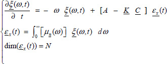
Consider the non-commensurate order fractional system

corresponding to the distributed differential system
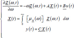
with
The objective is to estimate Ẕ(ω, t0), using the knowledge of {u(t), y(t)} on [tp, t0], with the constraint
Note that the system [3.4] is continuously distributed: it would be unrealistic to estimate the exact continuous distribution Ẕ(ω, t0).
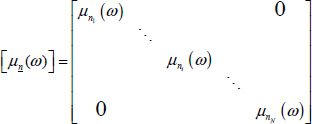
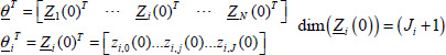
Practically, Ẕ(ω, t0) is approximated by its frequency discretized distribution (see Chapter 2 of Volume 1):
where for the ith fractional integrator
As stated previously, several techniques can be used to estimate Ẕ(t0). In fact, we propose to use the classical technique, i.e. the Luenberger observer, performing the estimation of Ẕ(t0) on the interval [tp, t0], where the observer would have to be ideally initialized by ![]() . Of course, since we have no prior knowledge of Ẕ(tp), the direct solution is to use
. Of course, since we have no prior knowledge of Ẕ(tp), the direct solution is to use
3.3. Initialization with a fractional observer
3.3.1. Fractional observer definition
There are many papers that deal with the Luenberger observer in the fractional order case [MAT 97, DZI 06, DAD 11, NDO 11]. In fact, these papers correspond to the estimation of the pseudo-state ![]() , not to the estimation of the internal state Ẕ(ω , t). Consequently, these fractional observers are only the generalization of integer order observers. Their requirements are the same as in the integer order case, except for stability.
, not to the estimation of the internal state Ẕ(ω , t). Consequently, these fractional observers are only the generalization of integer order observers. Their requirements are the same as in the integer order case, except for stability.
Thus, it is essential to note that in this section, we really analyze the observation of the internal state Ẕ(ω, t).
The theoretical initialization of an FDS at t = t0 concerns the estimation of its state z(ω, t0) based on the measurements of {u(t), y(t)} on a history interval [tp;t0]. Therefore, a direct way is to use a fractional observer.
Consider the FDS [3.3]. The Luenberger fractional observer [LUE 66, KAI 80, ZAD 08] is defined by
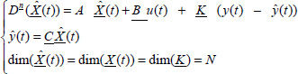
where ![]() and Ḵ are respectively the observer pseudo-state and the vector gain.
and Ḵ are respectively the observer pseudo-state and the vector gain.
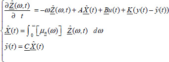
As for the FDS, we define the distributed state vector of the observer
and its representation (similarly to [3.4])
3.3.2. Stability analysis
Let us define the pseudo-state error
Then
Thus, from [3.9] and [3.11], we obtain
The stability of the FDS observer [3.9] depends on ![]() and ṉ, i.e. the observer gain Ḵ has to respect the stability of the estimation error.
and ṉ, i.e. the observer gain Ḵ has to respect the stability of the estimation error.
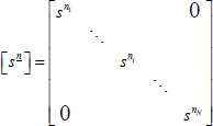
For a commensurate order system, the stability depends on the eigenvalues λi of the matrix ![]() and the value of the fractional order n (0 < n < 1). According to Matignon’s criterion [MAT 98], these eigenvalues have to verify the following condition (see also Appendix A.8.2):
and the value of the fractional order n (0 < n < 1). According to Matignon’s criterion [MAT 98], these eigenvalues have to verify the following condition (see also Appendix A.8.2):
For a non-commensurate order system, the stability condition is more complex to derive. For this purpose, we can use the technique proposed in Chapter 6, which is derived from the Nyquist criterion [NYQ 32, TRI 09c].
For example, consider the two-derivative system:
Let us define the transfer function
where
and
![]() is the well-known characteristic polynomial [KAI 80, ZAD 08] corresponding to the system [3.16, 3.17] which is of the form
is the well-known characteristic polynomial [KAI 80, ZAD 08] corresponding to the system [3.16, 3.17] which is of the form
Thus, the estimation error will be stable if ![]() is stable, i.e. if α0 > 0 and α1 > 0 (according to the Nyquist stability criterion in Chapter 6).
is stable, i.e. if α0 > 0 and α1 > 0 (according to the Nyquist stability criterion in Chapter 6).
3.3.3. Convergence analysis
Since ![]() is only the pseudo-state error, it is necessary to associate a distributed state variable error ξi(ω, t) with each component εx, i(t) of
is only the pseudo-state error, it is necessary to associate a distributed state variable error ξi(ω, t) with each component εx, i(t) of ![]() .
.
Thus, equivalent to [3.12] and [3.14], and taking into account [3.11], the distributed state vector error ![]() verifies the following equation (note that
verifies the following equation (note that ![]() does not correspond to the open-loop distributed state in this section):
does not correspond to the open-loop distributed state in this section):
Using [3.14] and [3.21] leads to
or
where ![]() is the state vector error.
is the state vector error.
The observer starts at t = tp, and it is supposed to be at rest at this instant because we have no information on Ẕ(ω, tp).
Therefore
Thus, [3.23] leads to
In order to simplify the notations, let us consider the reduced time
Then, the Laplace transform of [3.21] leads to
with
Therefore
and
This result means that
Thus, we can conclude that all the components of ![]() converge to those of Ẕ(ω, t) as t → ∞.
converge to those of Ẕ(ω, t) as t → ∞.
Nevertheless, the dynamics of ![]() are imposed by 1/(s + ω) (see [3.30]). Thus, the lower frequency modes of Ẑ(ω, t) require an infinite time to converge. Consequently, the requirement for convergence ∀ ω is that t0 – tp → ∞.
are imposed by 1/(s + ω) (see [3.30]). Thus, the lower frequency modes of Ẑ(ω, t) require an infinite time to converge. Consequently, the requirement for convergence ∀ ω is that t0 – tp → ∞.
3.3.4. Numerical example 1: one-derivative system
Consider the transfer function
Therefore, A = –a0, Ḇ = 1 and ![]() .
.
At t = 0, the system is at rest, i.e. z(ω, 0) = 0∀ω, x(0) = 0 and y(0) = 0.
The input of the system is a unity step on [0, t0]:
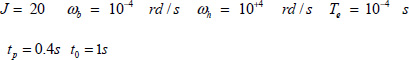
The past history interval corresponds to tp = 0.5s and t0 = 2s.
We simulate the system response y(t) with
The observer starts at t = tp with K = 20 and ẑ(ω, tp) = 0∀ω.
At t = t0, the initial state is z(ω, t0), whereas the initial state of the observer is ẑ(ω, t0). Then, at t = t0, we switch off the observer (K = 0). Consequently, its response represents the free response of the system initialized with the estimated initial condition ẑ(ω, t0), which we call the initialized response yinit(t).
The input u(t), the theoretical system response y(t), the observer response ŷ(t) and the initialized response yinit(t) are plotted on [0, 3t0] in Figure 3.1.
We can note that the observer response ŷ(t) is quickly close to y(t). However on [t0, 3t0], yinit(t) is progressively different from y(t). The first conclusion is that the equality of the pseudo-states (x(t) and ![]() at t = t0 is not a guarantee for a good initialization.
at t = t0 is not a guarantee for a good initialization.
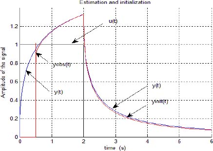
Figure 3.1. Input u(t) and outputs y(t), ŷ(t) and yinit(t). For a color version of the figures in this chapter see www.isteco.uk/trigeassou/analysis2.zip
The comparison between the components zj(t0) and ẑj(t0) (for j = 0,…, 20) provides the explanation of this difference (see Figure 3.2): the high frequency modes are correctly estimated, whereas there is a poor estimation of the very low frequency modes. Consequently, the initialization of the fractional system is poor for long time behaviour, as highlighted on [t0, 3 t0] (Figure 3.1).
REMARK 1.– The increase in the observer gain K shows that there is some improvement of the convergence of low frequency modes. Therefore, very large values of K (because stability is not theoretically affected) would theoretically improve convergence. In fact, a practical value Kmax is imposed by the numerical computation of the observer: note that the fractional integrator is approximated by a finite dimension model, and each mode is time discretized.
Thus, observer stability has to respect a more restrictive condition K < Kmax. Consequently, there is no simple solution to the improvement of the convergence of low frequency modes.
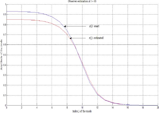
Figure 3.2. Comparison between modes zj(t0) and ẑj(t0) for j = 0,1,2,…, 20
3.3.5. Numerical example 2: non-commensurate order system
Consider the transfer function

corresponding to the observer canonical form [KAI 80]:
The values of the gain Ḵ have to be chosen to respect observer stability. Using the stability criterion of section 3.3.2, theoretical stability is ensured for K1 ≥ 0 and K2 ≥ 0.
The simulation protocol is the same as previously with
The graphs of u(t), y(t) and ŷ(t) for different values of Ḵ are presented in Figure 3.3.
Figures 3.4 and 3.5 present the graphs of the corresponding modes of ![]() and
and ![]() .
.
Obviously, the best estimation of Ẕ(t0) is provided by  . Nevertheless, the low frequency modes exhibit a poor convergence, as in the previous example.
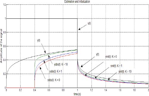
Figure 3.3. u(t), y(t), ŷ(t) and yinit(t)

Figure 3.4. Comparison between modes z1, j(t0) and ẑ1, j(t0) for j = 0,1,2,…, 20
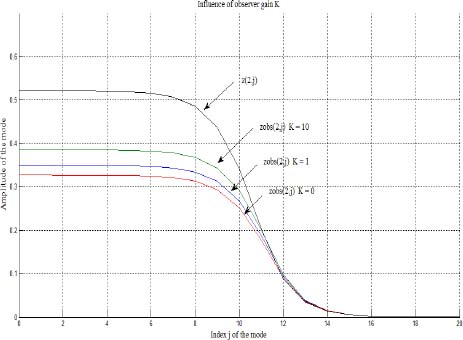
Figure 3.5. Comparison between modes z2, j(t0) and ẑ2, j(t0) for j = 0,1,2,…, 20
3.4. Improved initialization
3.4.1. Introduction
The previous convergence analysis demonstrated that the lower frequency modes of Ẕ(ω, t0) are not correctly estimated because they require an infinite history interval [tp, t0] for complete convergence. Obviously, this requirement is not acceptable in practice. A straightforward approach to improve Ẕ(ω, t0) estimation would be to artificially broaden the interval [tp, t0] by repeated forward/backward observations. This technique has been successfully used for the initialization of a PDE (see [RAM 10] and the references therein) where the direct model ![]() is used to perform forward observation, whereas the backward model
is used to perform forward observation, whereas the backward model ![]() is used to perform backward observation
is used to perform backward observation
Unfortunately, the application of this methodology to a fractional system is forbidden by numerical problems due to the fractional backward model [BOU 67]. This model is very sensitive to numerical errors that affect the high frequency modes. Apparently, this iterative procedure cannot be used with a fractional system.
However, this approach demonstrates that the improvement of Ẕ(ω, t0) estimation depends on the quality of the initial value ![]() of the observer.
of the observer.
Thus, we propose a solution to estimate Ẕ(ω, tp) using a fixed history interval [tp, t0] and the free response of the system starting at t = tp. As demonstrated thereafter, this estimation makes it possible to initialize the observer and then to improve the estimation of Ẕ(ω, t0).
The estimation of Ẕ(ω, tp) is based on a gradient approach using the open-loop responses ![]() of the fractional integrators
of the fractional integrators ![]() (closed-loop representation).
(closed-loop representation).
As demonstrated thereafter, ![]() is deduced from the free response of the system yfree(t). Since y(t) = yfree(t) + yforced(t), the free response yfree(t) is calculated from the knowledge of y(t) on [tp, t0] and on the simulation of yforced(t) based on the knowledge of u(t) on [tp, t0] and of the system parameters.
is deduced from the free response of the system yfree(t). Since y(t) = yfree(t) + yforced(t), the free response yfree(t) is calculated from the knowledge of y(t) on [tp, t0] and on the simulation of yforced(t) based on the knowledge of u(t) on [tp, t0] and of the system parameters.
3.4.2. Non-commensurate order principle
Let us consider the Laplace transform of the system response [3.3, 3.4] (see Chapter 7 of Volume 1):
where the first term represents the free response of the system initialized by Ẕ(ω, 0), and the second term represents the forced response depending only on the input u(t).
Let us define
and
Then
Since we consider the free response initialized by Ẕ(ω, tp), we obtain
As noted previously, the simplification of notations is based on the reduced time variable t – tp = t; therefore, Ẕ(ω, tp) = Ẕ(ω, 0).
Then
Practically, we use the frequency discretized model (see Chapter 2 of Volume 1); thus, we replace Ẕ(ω, 0) (in fact, Ẕ(ω, tp)) with
and ![]() with
with
where
Therefore, ![]() is linear in the parameter vector
is linear in the parameter vector ![]() .
.
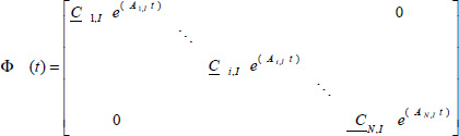
Note that in [3.45], Ai, I is diagonal; thus, the matrix Φ(t) is easily computed using Ai,I and Ci,I.
As demonstrated thereafter, we can compute the free response of the system yfree(t) for t ∈ [tp, t0] (see sections 3.4.3.1 and 3.4.3.2).
Therefore, expressing ![]() in terms of yfree(t) on the history interval, we can estimate
in terms of yfree(t) on the history interval, we can estimate ![]() as follows.
as follows.
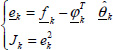
Let us define
where ![]() is an estimation of
is an estimation of ![]() . f(t) and
. f(t) and ![]() are known functions on [tp, t0] (see the illustrative examples given in sections 3.4.3.1 and 3.4.3.2).
are known functions on [tp, t0] (see the illustrative examples given in sections 3.4.3.1 and 3.4.3.2).
Note that the least-squares technique [EYK 74, NOR 86], based on the quadratic criterion ![]() , requires a matrix inversion that cannot be performed since the eigenvalues’of this matrix are distributed from 0 to + ∞, due to the wide range of ωj modes (see Chapter 4 for an analysis of this problem).
, requires a matrix inversion that cannot be performed since the eigenvalues’of this matrix are distributed from 0 to + ∞, due to the wide range of ωj modes (see Chapter 4 for an analysis of this problem).
Consequently, the gradient technique [RIC 71, LJU 87, TRI 88] is more appropriate as it does not require matrix inversion.
3.4.3. Gradient algorithm
Consider the quadratic criterion
Let t – tp = k Te (with Te being the sampling time, k ∈ N) and ![]() be the estimation at t = k Te. Thus,
be the estimation at t = k Te. Thus,
Using the online gradient algorithm [LJU 87], the new estimation ![]() at (k + 1) Te corresponds to
at (k + 1) Te corresponds to
or
The gradient algorithm presents two known drawbacks [RIC 71, TRI 88]: its stability depends on λ and it is highly sensitive to measurement noise, which imposes a low value of λ. On the contrary, in a deterministic context, convergence is relatively fast (with a high value of λ respecting λ < λmax). Moreover, it provides a confident estimation of Ẕ(ω, tp) without performing matrix inversion [TAR 16c, MAA 17].
Practically, several sequences of the gradient algorithm are necessary (one sequence corresponding to tp → t0), initialized at the first sequence by ![]() (see Appendix A.3. for convergence and stability of the gradient algorithm).
(see Appendix A.3. for convergence and stability of the gradient algorithm).
3.4.3.1. Example 1
Consider the transfer function system
Thus, ![]() .
.
Relation [3.51] leads to
Let us define
Then
and using [3.44]
Then, we can express
with
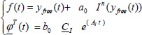
In(yfree(t)) corresponds to the fractional integration of yfree(t), which can be easily computed (see Chapter 2 of Volume 1).
Then, using the gradient algorithm [3.42], we can estimate ![]() .
.
3.4.3.2. Example 2
Consider the transfer function system
Thus, ![]() .
.
The calculation of yfree(t) and ![]() is based on the observer canonical form [KAI 80]:
is based on the observer canonical form [KAI 80]:
After simple calculations, relation [3.40] provides
which leads, in the time domain, to
Thus, from [3.44], we obtain
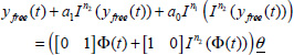
or

where
![]() corresponds to the first fractional integrator (with order n1), and
corresponds to the first fractional integrator (with order n1), and ![]() corresponds to the second integrator (order n2).
corresponds to the second integrator (order n2).
Then, we obtain

The fractional integrals In2(.) and In1(In2(.)) are easily computed using the frequency discretized model of the fractional integrators (see Chapter 2 of Volume 1). Thus, ![]() can be estimated by the gradient algorithm [3.49].
can be estimated by the gradient algorithm [3.49].
Of course, the regressor ![]() is more complex than in the first example, but it does not introduce numerical difficulties.
is more complex than in the first example, but it does not introduce numerical difficulties.
3.4.4. One-derivative FDE example
3.4.4.1. Introduction
Let us consider the system [3.51]:
Since the direct observation of the system state does not provide a confident estimation ẑ(ω, t0) (see section 3.3.4), we use the previous gradient technique to estimate z(ω, tp).
In Figure 3.6, we plot the step response y(t) starting at t = 0 and the corresponding free response yfree(t) starting at tp = 0.5 s. This simulation makes it possible to provide the required data {fk} of [3.55].
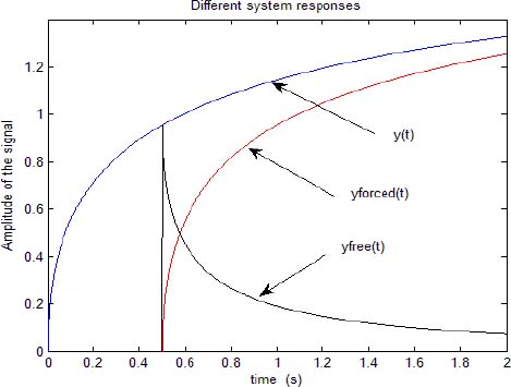
Figure 3.6. The different responses of the system on [0, t0]
3.4.4.2. Estimation tests of z(ω, tp)
The previous gradient algorithm is used to estimate z(ω, tp) with ![]() (which ensures algorithm stability).
(which ensures algorithm stability).
In Figure 3.7, we plot the frequency discretized components zj(tp) and ẑj(tp) obtained after several sequences. After one sequence, the estimation is poor, particularly for the higher modes. Therefore, it is necessary to perform several sequences of the gradient algorithm to improve this estimation. We note an improvement for five sequences, and an important one at the low and medium frequencies for 10 sequences.

Figure 3.7. Gradient technique estimation of modes ẑj(tp) for different sequences
3.4.4.3. Estimation of z(ω, t0)
The estimation ẑ(ω, tp) obtained after 10 sequences is selected to initialize the observer, and we keep the same gain K = 20 as with the previous direct approach.
In Figure 3.8, we plot zj(t0) (exact), ẑj(t0) (direct) and ẑj(t0) initialized by ẑj(tp) (improved).
The improvement of z(ω, t0) estimation is now significant, whereas ẑ(ω, t0) (direct) is far from z(ω, t0) at low frequencies, ẑ(ω, t0) (initialized by ẑ(ω, tp)) is excellent at all frequencies. Thus, the initialization of the one-derivative fractional order model is now excellent (Figure 3.9).
As we cannot objectively appreciate the initialization improvement, we compute the difference between the true response y(t) and its initialization yinit(t), i.e.
In Figure 3.10, we plot the direct initialization error and the improved initialization error. Obviously, the proposed methodology provides an important improvement to the initialization problem.

Figure 3.8. Direct and improved estimation ẑj(t0) for j = 0,1,2,…, 20
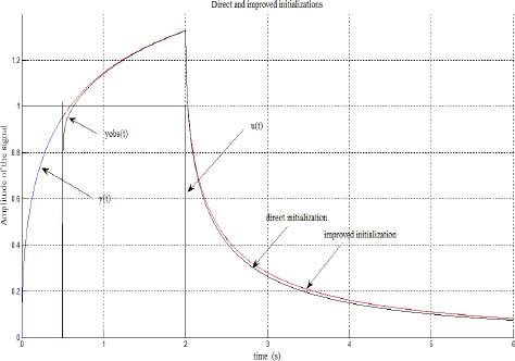
Figure 3.9. u(t), ŷ(t) (direct), ŷ(t) (improved) and yinit(t)
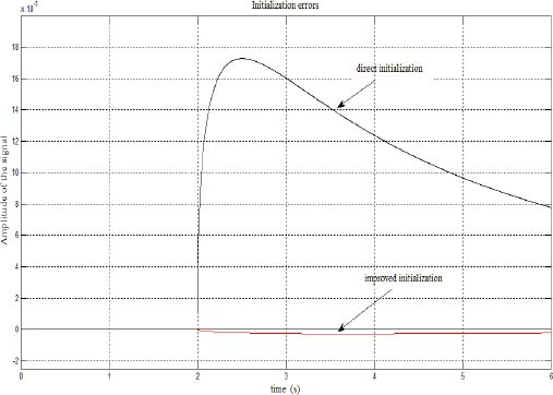
Figure 3.10. Comparison of initialization errors
3.4.5. Two-derivative FDE example
Let us consider again the non-commensurate example [3.58]:
In Figure 3.11, we present the step response y(t) starting at t = 0 and the corresponding forced response yforced(t) and free response yfree(t) starting at tp = 0.4s. This simulation makes it possible to provide the required data {fk} of [3.61].
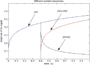
Figure 3.11. The different responses of the system on [0, t0]
3.4.5.1. Estimation tests of z(ω, tp)
The previous gradient algorithm was used to estimate  with
with ![]() and
and ![]() (which ensure algorithm stability).
(which ensure algorithm stability).
In Figures 3.12 and 3.13, we respectively plot z1, j(tp) and z2, j(tp) estimates for several sequences.
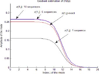
Figure 3.12. Gradient estimation of the modes ẑ1,j(tp) for different sequences
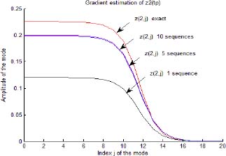
Figure 3.13. Gradient estimation of the modes ẑ2, j(tp) for different sequences
3.4.5.2. Estimation of Ẕ(ω, t0)
The observer is initialized with the estimation ![]() obtained after 10 sequences; moreover, it operates with the gain
obtained after 10 sequences; moreover, it operates with the gain  on the history interval [tp , t 0].
In Figures 3.14 and 3.15, we plot Ẕ(t0) exact, ![]() direct and
direct and ![]() initialized by
initialized by ![]() respectively for Ẕ1(t0) and Ẕ2(t0).
respectively for Ẕ1(t0) and Ẕ2(t0).
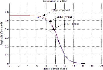
Figure 3.14. Direct and improved estimations ẑ1, j(t0)
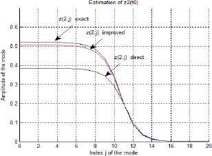
Figure 3.15. Direct and improved estimations ẑ2, j (t0)
As shown in these figures, ![]() improved by the gradient technique is now closer to Ẕ(ω, t0) exact, as in the previous example.
improved by the gradient technique is now closer to Ẕ(ω, t0) exact, as in the previous example.
Finally, in Figure 3.16, we compare the system response initialized by ![]() improved and by
improved and by ![]() direct. As shown by the comparison of initialization errors in Figure 3.17, the improved initialized response fits very well with the exact system response, and there is no longer the difference caused by the low frequency modes that characterize the direct initialization.
direct. As shown by the comparison of initialization errors in Figure 3.17, the improved initialized response fits very well with the exact system response, and there is no longer the difference caused by the low frequency modes that characterize the direct initialization.
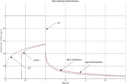
Figure 3.16. u(t), y(t), y(t) (direct) and ŷ(t) (improved)

Figure 3.17. Comparison of initialization errors
A.3. Appendix
A.3.1. Convergence of gradient algorithm
A.3.1.1. Asymptotic convergence
The gradient algorithm is expressed as
where ![]() .
.
Therefore
Assume that the algorithm converges to a value ![]() , then
, then ![]() .
.
Therefore
Since ![]() , the algorithm converges to
, the algorithm converges to
Of course, this property is classical: the least-squares technique is characterized by ![]() because the model is linear in the parameters [LJU 87].
because the model is linear in the parameters [LJU 87].
A.3.1.2. Convergence rate
In fact, convergence is not sufficient, and the convergence rate is more important in our case.
First, consider a one-parameter θj algorithm, with
As J(t) = e2(t), we obtain:
Therefore
This algorithm is stable if
First, consider the case ![]() . Then,
. Then, ![]() remains close to 1 even for large values of k.
remains close to 1 even for large values of k.
Therefore
Then, if λ is chosen as ![]() , convergence is fast and θj, k = θj is obtained with a few iterations.
, convergence is fast and θj, k = θj is obtained with a few iterations.
Then, consider the case ![]() . Then,
. Then, ![]() decays quickly and
decays quickly and ![]() with a few iterations. Therefore, θj,k = θj,k+1, and convergence is stopped far from θj.
with a few iterations. Therefore, θj,k = θj,k+1, and convergence is stopped far from θj.
Consequently, convergence requires several sequences of the gradient algorithm, because the variation of θj, k is possible only for the low values of k.
Then, consider the two-parameter case.
φ1(t) = c1 e–ω1t and φ2(t) = c2 e–ω2t with ω2 ≫ ω1.
Te is chosen close to ![]() , whereas
, whereas ![]() .
.
Therefore, φ2(t) decays quickly with k, whereas φ1(t) remains close to 1.
With the approximation φ1 ≈ 1, after a few iterations, the algorithm is equivalent to
This means that θ1, k converges to θ1, whereas θ2, k is blocked to a value different from θ2.
Consequently, θ1, k converges immediately, whereas several sequences are necessary for θ2, k convergence, as mentioned previously.
This result is easily generalized to a large number of parameters ![]() .
.
Parameters characterized by Te close to ![]() (high frequency modes) converge slowly, whereas low frequency modes converge quickly.
(high frequency modes) converge slowly, whereas low frequency modes converge quickly.
A.3.2. Stability and limit value of λ
Equations [3.69, 3.70] can be written as
Stability of [3.79] is conditioned by the eigenvalues µj(k) of A(k), with the requirement
for N = 1, we obtain ![]() ,
,
therefore
Practically, λmax decays with ![]() .
.
However, since λ is weighted by ![]() (i.e.
(i.e. ![]() ), the algorithm becomes increasingly stable as k increases (because λ(k) → 0).
), the algorithm becomes increasingly stable as k increases (because λ(k) → 0).