Chapter 11: Operational Excellence – Monitoring, Optimization, and Troubleshooting

In this chapter, we will focus on operational excellence. Operational excellence in this chapter has three components: monitoring Athena to ensure it is healthy and running normally, optimizing our usage of the system for cost and performance, and, lastly, how to troubleshoot issues when they occur.

When monitoring systems, it is essential to know what to monitor and what steps to take when something goes wrong. This information is valuable because when the system is not operating correctly, the data will give you clues on possible issues, which reduces investigation time. You can also act before problems occur, preventing calls from users on why things are not working. We will look into processes that can be put in place to ensure that Athena and our usage of it are normal and efficient. When there are issues, we will know how to fix common problems.

We also want to get the most out of Athena. To run optimally and cost-effectively, we will optimize our use of Athena by going through best practices on how to store our datasets and best write queries. Following these best practices can significantly reduce your monthly bills and keep your users happy, with low query times.

Lastly, we will look at how we can troubleshoot failing queries. We will dive deep into the most common problems users encounter, what they mean, and how to address them.

In this chapter, we will learn about the following:

• How to monitor Athena to ensure queries run smoothly
• How to optimize for cost and performance
• How to troubleshoot failing queries

Technical requirements

For this chapter, if you wish to follow some of the walk-throughs, you will require the following:

• Internet access to GitHub, S3, and the AWS Management Console.
• A computer with a Chrome, Safari, or Microsoft Edge browser installed.
• An AWS account and accompanying IAM user (or role) with sufficient privileges to complete this chapter's activities. For simplicity, you can always run through these exercises with a user that has full access. However, we recommend using scoped-down IAM policies to avoid making costly mistakes and to learn how to best use IAM to secure your applications and data. You can find a minimally scoped IAM policy for this chapter in the book's accompanying GitHub repository, listed as chapter_11/iam_policy_chapter_11.json (https://bit.ly/3hgOdfG). This policy includes the following:
  • Permissions to read, list, and write access to an S3 bucket
  • Permissions to read and write access to the AWS Glue Data Catalog databases, tables, and partitions:
    • You will be creating databases, tables, and partitions manually and with Glue crawlers.
  • Access to run Athena queries

Monitoring Athena to ensure queries run smoothly

Monitoring your usage of Athena is essential to ensuring that your users' queries continue to run uninterrupted without issues. Many issues can be addressed before they impact users and applications. This section will look into the metrics that Athena emits to CloudWatch Metrics and the metrics that should be monitored and alarmed on, so that actions can be taken before users reach out to their administrators. Before we do, let's take a look at which metrics are emitted by Athena.

Query metrics emitted by Athena

Athena emits query-level metrics for customers to be able to monitor and alarm on. These metrics exist in CloudWatch Metrics under the namespace "AWS/Athena" and three dimensions, QueryType, QueryState, and the Workgroup name. QueryType can be DML (INSERT/SELECT queries) or DDL (metadata queries such as CREATE TABLE). QueryState can be SUCCEEDED, FAILED, QUEUED, RUNNING, or CANCELED. The Workgroup dimension aggregates metrics within the Athena workgroup that the query executed in.

The metrics that are emitted are listed here:

• TotalExecutionTime – in milliseconds. The entire execution time of the query from when the query is accepted by Athena to when it reaches its final state (SUCCEEDED, FAILED, or CANCELED).
• QueryQueueTime – in milliseconds. This is the time a query spent waiting for resources to run on. This measures the time after Athena has accepted a query for execution and before it is sent to the execution engine for execution.
• EngineExecutionTime – in milliseconds. This is the amount of time taken when the query is received by the execution engine to when it completes executing it. This metric includes the QueryPlanningTime metric. This applies to both DML and DDL queries.
• QueryPlanningTime – in milliseconds. This is the amount of time the execution engine (that is, PrestoDB) took to parse the query and create its execution plan. This includes operations such as retrieving partition information from the metastore, optimizing the execution plan, and so on. This applies to DML queries only.
• ServiceProcessingTime – in milliseconds. This is the time from when the query has finished in the execution engine (that is, PrestoDB) and the time Athena uses to read the results and push them to S3. This applies to both DML and DDL queries.
• ProcessedBytes – in megabytes. This is the amount of data that the execution engine processed for DML (that is, SELECT) queries. This can be used as an approximation for billing.

With these metrics, we can build dashboards and alarms. The process to create the alarms will be included in the following sections.

Monitoring query queue time

To protect available resources for all customers, Athena allows a certain number of queries to be run at any given time from a single AWS account. When a query is submitted for execution, Athena will check how many queries the submitting account is executing. If it exceeds the account limit, or if there are not enough resources, say at peak times during the day, then the query will be queued until both of those conditions are met. When clients submit their queries and notice that their queries are not running or taking a significant time to run even a small query, it is likely because they are queued.

Monitoring and actioning when Athena queue time occurs is essential to prevent users' queries from being constantly queued. Since queue time metrics are emitted to CloudWatch metrics, alarms can be created and actioned against. We have included a sample script that can be used as templates to monitor and email when thresholds are exceeded, which can be found in this chapter's GitHub location at https://bit.ly/3j7Nzly. The script can be adjusted for your use case. It will create four alarms, two for DML queries and two for DDL queries. Each set will generate a warning threshold and one for when production impact occurs. The split between DML and DDL queries is due to the query types having their own queues, and one will not impact the other.

Once the alarms are created, then the CloudWatch alarms dashboard may look like the following.

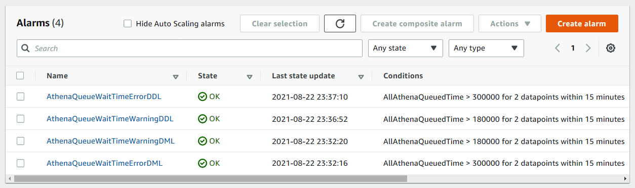
Figure 11.1 – A sample alarm dashboard in Amazon CloudWatch for alarms

When users' queries start to get significantly queued, three actions can be taken. First, reduce the frequency that queries are submitted or spread them out throughout the day. This can be done by asking users or by disabling low-priority users. This is not an ideal solution but can be a short-term solution to prioritize applications or users that need to execute queries. The second action that can be taken is to submit a support case and ask for the AWS account to increase concurrent query execution for your AWS account. This generally happens automatically but is not done when there is a sudden increase in sustained usage. Requests to increase query concurrency need to be considered by AWS and may be approved or disapproved.

The last solution is to split queries among AWS accounts. This approach has the additional benefit of isolating applications and users from impacting each other. It is best practice to use an AWS account for SLA-sensitive applications and users, and other ad hoc queries from users doing data exploration in another account.

Let's now look at monitoring Athena's costs.

Monitoring and controlling Athena costs

No one wants to be emailed or especially called because their team's Athena costs are significantly higher than initially expected. Unexpected increases in costs can be due to a single user running a query without a partition filter that unintentionally scans terabytes of data or an application with a bug that makes an unexpectedly high number of calls. There are mechanisms that Athena provides to prevent these scenarios when using Athena workgroups.

To prevent the scenario of a single user running every large and expensive query, workgroups can be configured to cancel individual queries that exceed a quantity of data read. This is configurable for each workgroup, depending on the need. To set this feature, go to the Data usage controls tab when editing a workgroup in the Athena console, as shown in the following figure:

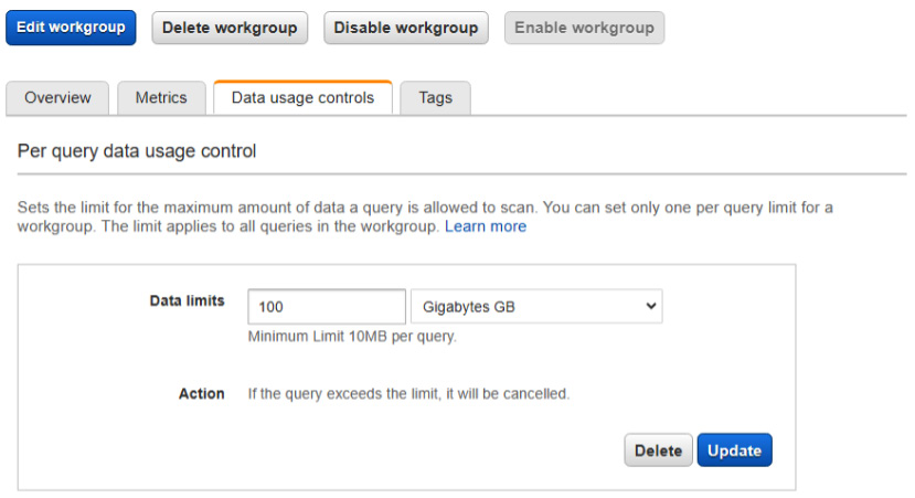
Figure 11.2 – Data usage controls within the Athena console for a workgroup

Within this tab, you can set data usage limits at a query level. By selecting this limit, Athena will cancel queries that exceed the query limit. It is recommended that this limit be configured to a value that prevents legitimate queries from being interrupted but is low enough to identify issues.

In addition to setting limits at a query level, you can also set ProcessedBytes limits at a workgroup level. CloudWatch alarms can be created in CloudWatch or through the Athena console in the workgroups tab, as shown in the following figure:

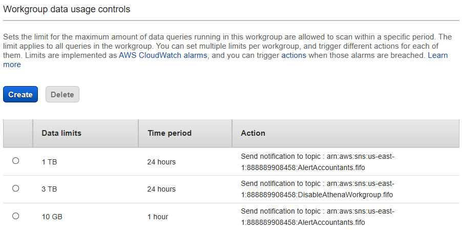
Figure 11.3 – Workgroup data usage controls section below per query limits

The previous figure shows an example in which three alarms notify different Amazon SNS topics in which different actions can be taken. This is an example where warning emails can be sent out to interested parties if the usage and cost exceed certain thresholds. The other two thresholds can disable the workgroup. Going above 3 TB of usage would be considered highly unusual for this use case, and an investigation should be done.

The above example alarms were created by clicking the Create button in Figure 11.2. As seen in Figure 11.3, the window that pops up allows data limits and a time period to be entered, and an optional SNS queue to send a notification to. Each alarm created is backed by a CloudWatch alarm and can be tweaked through the CloudWatch alarm console.

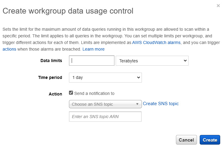
Figure 11.4 – Creating a workgroup data usage alarm

Now that we have seen how to monitor and put limits on query usage, let's look at how we can optimize using Athena to reduce costs and query runtime.

Important Note

If you are using the federated connectors, you will incur costs associated with the connectors, such as the cost of launching Lambda functions and the resources used when running Lambda.

Optimizing for cost and performance

When optimizing performance for any execution engine, two goals should always be kept in mind: read as little data from your storage as possible, which reduces costs and reduces query time, and make sure that your query engine does as little work (processing) as possible, which reduces query time.

This section will look similar to the AWS Big Data Blog post titled Top 10 Performance Tuning Tips for Amazon Athena (https://amzn.to/2VIFv1y) that I wrote. Still, we will provide some additional details that the blog post did not offer. Many customers bookmark this page and refer to it, and I recommend visiting it often to improve its view count.

Important Note

The recommendations in this section are generalizations and may not apply to all circumstances. Everyone's data, data structure, and queries are different, so not all of these recommendations may drive an improvement. Testing and prototyping are highly recommended when going through the process of optimizing usage.

Let's get started by looking at some optimizations on how to efficiently store data.

Optimizing how your data is stored

It is essential to consider how your data is stored when being read by execution engines such as Athena. How your data is stored usually has the most significant impact on how queries perform and how much they cost. Also, if you need to regenerate data when your system is live, it is much more expensive than doing it upfront. Changing queries is much easier and cheaper. With this in mind, some planning and prototyping are highly recommended.

Let's look at how file sizes and count impact performance.

File sizes and count

The size and number of files have a pretty significant impact on the performance of your Athena queries.

Important Note

The general recommendation is that your file sizes are between 128 Mb and 1 GB.

There are many reasons for this:

• S3 list operations are expensive. If you have a high number of files for a table, more S3 list operations need to be performed to get the list of files to read for a dataset.
• For each file, the engine needs to perform many S3 operations to consume it. It will first need to open the file by running a HeadObject() function to get the file size, encryption keys, and any other information necessary to start reading the file. This operation is expensive. Next, it will need to call a GetObject() function that returns a pointer to the data and the first data block. Ideally, you want to minimize the overhead of calling the HeadObject() function.
• The smaller your files, the less effective the compression, increasing the total amount of data stored.
• If your files are encrypted using server-side encryption, S3 will need to call the AWS KMS service to get decryption keys. This introduces overhead and increases costs because KMS charges for each call. I had a customer where their KMS costs were higher than their Athena costs because the cost of getting KMS keys was higher than reading the data. Having larger files reduces the number of calls needed for encryption keys.

Having appropriate file sizes reduces the amount of work that the execution engine needs to do.

Compression

Using compression makes the engine read less than uncompressed data, reducing network traffic from the data source to the Athena engine. For S3, it reduces storage costs. There is a trade-off of CPU usage as compression requires extra work to decompress data. Still, this cost is most of the time outweighed by making fewer calls to S3, and most queries do not exhaust CPU resources.

Important Note

Always compress your data when using text-based file formats, such as JSON and CSV. If your file sizes are larger than 512 Mb, use a compression algorithm that allows for files to be splittable. When using Apache Parquet or Apache ORC, compression should be applied within the column blocks (not to be confused with compressing the entire file).

When trying to decide on a compression algorithm, there are two aspects to consider. First, there is a trade-off between higher compression ratios and higher CPU usage. Second, whether the compression algorithm allows a query engine to read different parts of a file without reading the entire file. This is called if the file is splittable. If the algorithm produces splittable files, then multiple readers can read the file simultaneously, which increases parallelism. If a file is not splittable, a single reader must read the entire file, reducing parallelism.

For text-based file formats, such as JSON and CSV, it's always recommended to compress them because the compression ratios are generally very high. For columnar formats such as Apache ORC and Apache Parquet, they support compressing column data blocks. Because compression works best when groups of similar values exist, compressing all the values for a column in a single block usually leads to better compression ratios. Typically, Parquet and ORC are configured to compress column blocks by default.

File formats

Data formats impact the amount of data that a query engine reads and the amount of work the engine needs to do to read the data contained in the files. If your data is not in an optimal format, then transforming the data may reduce your overall cost if the cost of transformation is less than the cost of querying the data.

Important Note

For datasets that are read frequently, use Apache Parquet or Apache ORC. For data that is not likely to be queried or is queried infrequently, any compressed file format should be used. Datasets stored in CSV or JSON that will be queried frequently should be transformed into Parquet or ORC.

Let's dive into some common file formats.

• Row formats: CSV and JSON formats are the most common file formats used today but are the most inefficient. They are text-based, which is less efficient than storing the data in a binary format. For example, the int data type can be stored in binary using 4 bytes of data, but the number 1234567890 uses 10 bytes to store as a string. Add the delimiter for CSV and the field names in JSON, and they can take a substantial amount of space and memory. Also, when the file parser reads a number, it first needs to read the number as a string and then convert it to a number.
• Columnar formats: Columnar formats store data differently than row-based formats. With columnar formats, the data is grouped by the columns and stored in column blocks. A columnar file is then created by storing all the column blocks. When a reader wants to read the file, it will read each column block and generate a row by putting together all the columns by the index in the block. There are many reasons why this is cheaper and faster:
  • Field values are stored in binary instead of text. This reduces storage size and eliminates conversion from strings to numeric types, reducing the engine's read amount and work.
  • If a query only contains a subset of the columns, the execution engine will only read those columns, reducing the amount of data read.
  • Compression on blocks of data that contain similar values is generally more efficient. This reduces the amount of data needed to be read, which reduces the cost and work demanded from the engine.
  • Both Parquet and ORC support predicate pushdown, also known as predicate filtering. Parquet and ORC store statistics about each column block that can help skip reading entire blocks by pushing a filter to the reader and evaluating the filter on these statistics. If it is determined that the filter value is not in the data block, it is skipped. The statistics include ranges of values in the block and, for string data types, a Bloom filter. This reduces the cost and work demanded from the engine.

Parquet and ORC are better formats in almost every way than text-based formats. Let's take a look at how partitioning and/or bucketing your data can improve performance and costs.

Partitioning and bucketing

Partitioning and bucketing are two different optimizations that can lead to significant improvement in cost and performance. These features require an understanding of the data's usage patterns or how users or applications will query the datasets. Depending on the queries that will mainly be executed, it will inform the best way to leverage partitioning and bucketing.

Let's look at both features in a bit more detail:

• Partitioning: Partitioning your table separates rows into separate directories based on a column value. When a query contains a filter on a partition column value, only the partitions that meet the filter will be read, reducing the amount of data read. We talked about partitioned tables in Chapter 4, Metastores, Data Sources, and Data Lakes.

  Important Note

  Partitioning can significantly improve the performance and cost of your queries. A general recommendation for partitioning is to keep the number of partitions for a table under 100,000 while maintaining file sizes within the partitions.

  Choosing partition columns can be a challenge, but here are some best practices. When looking at the queries executed against the table, the columns in WHERE clauses are great candidates to look at. An example would be a dataset containing a transaction date. The date is in the WHERE clause very frequently because users only need the most recent data.

  The next best practice is to keep in mind the number of partitions your table has. The more partitions your table has, the smaller the files may be in each partition, which goes against file size best practice. Additionally, there is overhead when using partitioning, but if the partition column is chosen wisely, the overhead will be insignificant compared to the performance and cost savings. When Athena reads a partitioned table, it will need to fetch partition information from the metastore, and the greater the number of partitions, the more partitions it will need to fetch. A general recommendation is not to exceed 100,000 partitions, but this number depends on the upper bound of the query execution time and the amount of data in the dataset.

  One unique feature that Athena has that could help read tables with many partitions is partition projection. It allows tables to specify the partition columns and the expected values that those columns may take within the table properties. When Athena queries the partitioned table, it generates the partitions on the fly instead of going to the metastore to retrieve the partition information. This works for tables that store their partitions on S3 in a consistent directory structure, with partition columns whose values can be specified in a list or a range. Partition projection supports integer and string data types and supports date formats as well. You can see examples of partition projection using various datasets in this book at https://amzn.to/38a2FAC.

  Although not yet supported in Athena, one last optimization is indexing your Glue Data Catalog tables' partition data. When this feature is supported, it will significantly improve partition retrieval performance within Athena and reduce query time. Keep an eye out for when this is available.

• Bucketing: Bucketing is similar to partitioning because it groups rows with the same column values in a file within a partition. You specify the number of buckets you want at table creation time and the column to bucket on. The engine will then hash the bucket column values and put the rows with the same hash value in the same file. When a query engine has a filter for specific values for the bucketed column, it can then run the hash on filter values and determine which files it needs to scan. This could lead to entire files being skipped.

  Important Note

  Bucketing can significantly improve the performance and cost of your queries. However, bucketing adds complexity and should be employed by advanced users for the most time-sensitive workloads.

  The following diagram shows what the NYC taxi dataset may look like if bucketing is employed. The sample CREATE TABLE statement is located at https://bit.ly/3kjd4j9.

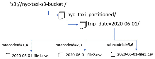
Figure 11.5 – An example of bucketing on the NYC taxi dataset

The dataset is partitioned by the trip_date value but bucketed on the ratecodeid column. All rows that contain the value in the ratecodid column of 1 and 3 will go into 2020-06-01-file1.csv, 2 and 3 will go into the 2020-06-01-file2.csv file, and 5 and 6 would go into the last file. If the query SELECT * FROM nyc_taxi_partitioned where ratecodeid = 3 is executed, Athena will determine that ratecodeid only existed in the 2020-06-01-file2.csv file and hence can skip the other two files. However, if the query SELECT * FROM nyc_taxi_partitioned where ratecodeid > 3 is executed, Athena will read all the files because it does not know the complete list of possible values.

There are some limitations to discuss. The current version of PrestoDB that Athena uses only supports tables that were bucketed using Hive, without the ability to insert data after a table or partition has been created. Once Athena offers a newer version of PrestoDB, this limitation may be removed and support Apache Spark's bucketing algorithm. Also, once the number of buckets is chosen for the dataset, it cannot be changed unless the entire dataset is regenerated. For these reasons, it is recommended that only advanced users attempt to leverage bucketing.

Now that we have gone through the optimization techniques to lay out our datasets on S3, let's look at some optimization techniques when writing queries.

Optimizing queries for performance

Although how data is stored can make the most significant impact on the performance of Athena queries, how queries are written is also important. In this section, we will go through some best practices when optimizing your queries.

Explain plans

Athena recently released a new feature that allows you to look at the execution plan of your queries. The execution plan is the set of operations that the engine performs to execute the query. It is not a requirement to read and understand the execution plans to optimize, but if we know how to read them, they can give us a valuable tool to dive deep into how queries are being executed. If you are not able to follow the technical details, it is okay. The other sections for optimizing your query will provide general recommendations that anyone can follow.

Let's take a quick look at an example of the information that EXPLAIN provides. If we take the simple query EXPLAIN SELECT SOURCE_ADDR, COUNT(*) FROM website_clicks GROUP BY source_addr, we get the following logical execution plan (edited to simplify the output):

Query Plan

- Output[SOURCE_ADDR, _col1] => [[source_addr, count]]

    - RemoteExchange[GATHER] => [[source_addr, count]]

        - Project[] => [[source_addr, count]]

            - Aggregate(FINAL)[source_addr][$hashvalue] => [[source_addr, $hashvalue, count]]

                - LocalExchange[HASH][$hashvalue] ("source_addr") => [[source_addr, count_8, $hashvalue]]

                    - RemoteExchange[REPARTITION][$hashvalue_9] => [[source_addr, count_8, $hashvalue_9]]

                        - Aggregate(PARTIAL)[source_addr][$hashvalue_10] => [[source_addr, $hashvalue_10, count_8]]

                            - ScanProject[table schemaName=packt_serverless_analystics_chapter_11, tableName=website_clicks, analyzePartitionValues=Optional.empty}] => [[source_addr, $hashvalue_10]]

                                    LAYOUT: packt_serverless_analystics_chapter_11.website_clicks

                                    source_addr := source_addr:string:1:REGULAR

This can look daunting at first, so let's break it down. The plan from the top down goes backward from the order of operations. The operation executed is ScanProject, which does the reading of our source data, our website_clicks table. The second operation is Aggregate, which does a partial GROUP BY function on the local node before sending it to the RemoteExchange operation. RemoteExchange shuffles data between the nodes of the partially aggregated data based on a hash code so that rows that contain the same GROUP BY columns go to the same node. LocalExchange shuffles data within a worker node. Then, a final Aggregate operation aggregates all the rows with the same GROUP BY values. The Project operator removes the hash code column and then performs the last RemoteExchange operation to a single node, to output the results using the Output operator.

To graph a visual representation of the plan, you can specify the format to GRAPHVIZ and use an online conversion tool to convert the output to an image. The one that is used within this chapter is https://dreampuf.github.io/GraphvizOnline/. The converted image for the query EXPLAIN (FORMAT GRAPHVIZ) SELECT SOURCE_ADDR, COUNT(*) FROM website_clicks GROUP BY source_addr is located at https://bit.ly/3yOMFzD.

If the type of execution plan is not specified, such as the previous example, a logical plan is provided. But Athena supports three other types of execution plans. They are VALIDATE, IO, and DISTRIBUTED, which can be specified in the query. For example, to validate whether a SQL statement is valid before executing it, you can run EXPLAIN (TYPE VALIDATE) <SQL STATEMENT>. It will return a true or false value, depending on whether Athena can parse and execute the query. The IO execution plan outputs the input and outputs of the query. An IO plan for the previous example can be seen at https://bit.ly/2VYnzjh.

The DISTRIBUTED plan provides fragments of the execution plan that is executed across different nodes. Each fragment is performed on one or more nodes depending on the type of the fragment. There are several fragment types, including SINGLE, HASH, ROUND_ROBIN, BROADCAST, and SOURCE. The SINGLE type of fragment executes only on a single node. The HASH type executes on a fixed number of nodes where the data is distributed among the nodes, based on a HASH code derived from one or more column values. For example, the source_addr column would be hashed for the previous query because it is in GROUP BY. To perform the GROUP BY function, rows with the same source_addr value need to be on the same node to do the aggregation. The ROUND_ROBIN type means that data is sent in a round robin to multiple nodes for operations such as transformations. The BROADCAST type means that the input of the fragment is the same across one or more nodes. This type is sometimes used with joins if a table is small enough to send to all nodes to do the join, which can significantly improve join performance.

Lastly, the SOURCE type specifies a fragment that reads from a source data store. In each fragment in the plan, the input data is determined by the RemoteSource[FragmentNumber] value, where FragmentNumber is the source fragment. To see the distribution plan for the previous query example, visit https://bit.ly/3g58Lqw.

Now that we have a basic understanding of how to read execution plans, let's look at some of the optimizations we can make to our queries, starting with optimizing joins.

Optimizing joins

The order in which tables are expressed in a join operation can significantly impact your query performance.

Important Note

When joining tables, order the largest tables on the left to the smallest tables on the right.

You may ask why the ordering of tables matters. Athena does not have access to statistics yet to reorder joins optimally as other database systems do. This may change in the future, but it is up to the user to perform this ordering for now.

For those interested in the technical details of why ordering matters, we need to understand how Athena performs joins. In summary, both tables get read and shuffled to a join operator to perform the join. However, there is an extra operation for the table on the right side. If the right-side table is smaller, the extra operation will be cheaper than if the operation occurred on the larger table. If we look at the explain plan for a query that performs a join, EXPLAIN (Type DISTRIBUTED) SELECT larger_table.table_data FROM larger_table LEFT OUTER JOIN smaller_table on larger_table.table_key = smaller_table.table_key, we see the following subsection of the distributed plan (the full explain plan can be found at https://bit.ly/37MH0hG):

Fragment 1 [HASH]

    Output layout: [table_data]

    Output partitioning: SINGLE []

    Stage Execution Strategy: UNGROUPED_EXECUTION

    - LeftJoin[("table_key" = "table_key_0")][$hashvalue, $hashvalue_9] => [[table_data]]

            Distribution: PARTITIONED

        - RemoteSource[2] => larger_table

        - LocalExchange[HASH]

            - RemoteSource[3] => smaller_table

The LocalExchange operator reshuffles the data within the worker. If the join order was reversed, the reshuffle would occur on the larger table, which would require more work and would cause the query to run longer.

Now let's look at optimizing the ORDER BY operator.

Optimizing ORDER BY

You will often need to order your results to get the top N number of results to generate reports or look at a subset of data when exploring a dataset. However, doing an ORDER BY operation on a large dataset can be a costly operation.

Important Note

When performing ORDER BY operations, using LIMIT can dramatically reduce query time if only the top N results are needed.

We need to understand why performing a global ordering requires a single worker to get the entire result set and perform a global sort, even if the input is sorted from many workers. Performing a global sort is very memory- and CPU-intensive. By limiting the number of results in the output, workers pushing rows to the global sort of an operator can limit the number of rows to it. The global sort can be done on a much smaller set of data. Let's look at the execution plan when LIMIT is specified for the query EXPLAIN SELECT total_amount FROM nyc_taxi where payment_type = 1 ORDER BY trip_distance LIMIT 100 (the full explain plan can be found at https://bit.ly/2VSMvc4):

Query Plan

- Output[total_amount] => [[total_amount]]

    - Project[] => [[total_amount]]

        - TopN[100 by (trip_distance DESC_NULLS_LAST)]

            - LocalExchange[SINGLE]

                - RemoteExchange[GATHER]

                    - TopNPartial[100 by (trip_distance DESC)]

                        - ScanFilterProject[table = nyc_taxi]

Without the LIMIT operator, the TopNPartial operator would not be in the plan. All results would go to the TopN operator. Performing the local sort before performing the RemoteExchange operation limits the amount of data shuffled, saving time and bandwidth.

Let's now look at the next best practice.

Selecting only the columns that are needed

This recommendation should be self-evident, but I have seen many customers not do this.

Important Note

Only select the columns in your query that are required as the output of your query.

There are many reasons why this can save both time and cost. For columnar data types, less data is read, which reduces cost. Another reason is that there is less data that needs to be shuffled between workers and outputted.

Let's now look at our last best practice.

Parallelizing the writing of query results

When Athena executes a SELECT query, the query's output is written by a single worker. If there is a huge result set, the amount of time to write the results from the single worker can be significant.

Important Note

For queries that produce a large number of results, use CTAS, INSERT INTO, or UNLOAD to parallelize the writing of the output.

Troubleshooting failing queries

When Athena works, it is excellent. It queries data in S3 without having to worry about servers or installing and maintaining software. But when Athena fails to execute a query, it can be tricky to know how and where to start looking. Issues can include how you wrote your query, problems with your metadata, or your data. In this section, we will go through some common failures and how to approach them. However, this list is not exhaustive. Athena's documentation publishes many error messages that customers see and how to deal with them, so bookmark it and refer to it when needed.

When your query starts failing, here is a list of actions that you can take:

• If your queries were working previously but are failing now, determine what has changed. Source control for queries that applications submit can help keep track of code and queries that have changed. If the queries have not changed, then most of the time, the issue is due to the loading of new data that it cannot process or metadata that was changed. This question is usually the first one that AWS Support would ask.
• Retry your query after a few minutes. Some failures with Athena are transient, such as when S3 throttles Athena because the load was too high on a particular S3 partition.
• Go to Athena's troubleshooting documentation, which contains a list of error messages and solutions (located at https://amzn.to/3kjBuJt).
• If all else fails, and you have access to AWS Support, then enter a support ticket. When creating a support ticket, the query ID and AWS region should be provided to help with the investigation. Providing a small sample of data is super helpful to AWS Support and the Athena development team to reproduce the issue. Just ensure that it does not contain any sensitive data.

Let's look at some common issues that customers face with Athena.

My query is running slow!

This is the most common issue that customers have when using Athena. Following the recommendations in the optimization section generally solves this issue. Using partitioning, converting to Apache Parquet or Apache ORC, and ensuring queries are optimally written will solve most of the reasons why queries may be running slow. If these do not, the other reason may be that too many concurrent queries are being run, and queries are being queued by the Athena service. You can check this by running your query and running a CLI command to get the amount of time the query spent in the queue. The following shows an example of the CLI command and its results:

aws athena get-query-execution --query-execution-id <EXECUTION ID>

{

    "QueryExecution": {

        "QueryExecutionId": "edea5091-6061-44bb-89ce-96090098c1b1",

        "Query": "select * from customers limit 10",

        "StatementType": "DML",

        ... (Section omitted ) ...

        "Statistics": {

            "EngineExecutionTimeInMillis": 511,

            "DataScannedInBytes": 35223,

            "TotalExecutionTimeInMillis": 765,

            "QueryQueueTimeInMillis": 155,

            "QueryPlanningTimeInMillis": 89,

            "ServiceProcessingTimeInMillis": 99

        },

        "WorkGroup": "packt-chapter11"

    }

}

Under the statistics section, you will see the QueryQueueTimeInMillis statistic. This value shows you the amount of time the query spent in Athena's queue, waiting for resources to execute on. If this value is consistently high, then your query rate is too high. Recommendations on how to monitor and the steps to correct this are in Monitoring query queue time in this chapter.

My query is failing due to the scale of data

This is the next most common issue customers face. The amount of data that Athena can scan is only limited to the maximum amount of time the query can run for, which by default is 30 minutes. When Athena performs simple table scans, it can process petabytes of data. However, if you see error messages such as INTERNAL_ERROR_QUERY_ENGINE, EXCEEDED_MEMORY_LIMIT: Query exceeded local memory limit, Query exhausted resources at this scale factor, and encountered too many errors talking to a worker node. The node may have crashed or be under too much load, then it's highly likely that your query contains complex operations, such as joins, aggregations, or windowing functions. These operations are performed by shuffling data around to nodes based on the values of the rows and stored in memory until the operation is completed. If a single node in the execution engine's cluster exhausts its resources, the query will fail.

There are a few strategies to overcome this issue. The first is to reduce the amount of data processed within the query by filtering data as soon as you read a table before complex operations. For example, take the following query:

SELECT upper(col1), sum(col1 + col2) FROM

    (SELECT

        table1.key, table1.col1, table2.col2

     FROM table1

     LEFT OUTER JOIN table2

     ON table1.key = table2.key) innerQuery

WHERE col2 > 10

This can be rewritten as follows:

SELECT upper(col1), sum(col1 + col2) FROM

    (SELECT

        table1.key, table1.col1, table2.col2

     FROM table1

     LEFT OUTER JOIN

        (select * from table2 WHERE col2 > 10)

     ON table1.key = table2.key) innerQuery

Filtering data before performing a complex operation can really improve performance and reduce memory requirements. Selecting only the columns that are of interest can help as well. Lastly, splitting up the query into smaller queries that scan a subset of partitions may help.

The other strategy is to find out whether your data has any data skews. Data skews exist when your data is not evenly distributed across a cluster when a complex operation is performed. For example, suppose there was a dataset that tracked all the different types of chairs. You performed a join on the number of legs a chair has to a dimension table, that is, SELECT * FROM chairs JOIN dim ON chairs.legcount = dim.legcount. Since most chairs have four legs, there will be significantly more data going to one node to perform the join, exhausting all the available memory. The only way to deal with this is to distribute the joins data across several nodes by joining on more than the legcount column or to reduce the number of rows by aggregating the data before the join occurs.

Now that we have gone through some troubleshooting techniques, let's summarize what we have learned in this chapter.

Summary

In this chapter, we went through best practices to get the most out of Athena while making sure it operates smoothly. We went through how we can create alarms to keep track of query queue time and costs, and take action to prevent Athena's unexpectedly high usage from leaving us with unexpected bills at the end of the month. We then went through how to optimize our usage of Athena by looking at best practices on how to store data and the queries we run. To do that, we explored how to look at the explain plans and how to read them to identify possible bottlenecks or issues with the written queries. Lastly, we looked at what to do when a query fails and the common problems users usually encounter.

The next chapter will dive into query federation, which allows you to query almost any data source with Athena.

Further reading

• Amazon Athena CloudWatch Metrics – https://docs.aws.amazon.com/athena/latest/ug/query-metrics-viewing.html
• Top 10 Performance Tuning Tips for Amazon Athena – https://aws.amazon.com/blogs/big-data/top-10-performance-tuning-tips-for-amazon-athena/
• Athena Partition Projection – https://docs.aws.amazon.com/athena/latest/ug/partition-projection.html
• Athena EXPLAIN documentation – https://docs.aws.amazon.com/athena/latest/ug/athena-explain-statement.html
• PrestoDB 0.217 EXPLAIN documentation – https://prestodb.io/docs/0.217/sql/explain.html
• Amazon Athena Troubleshooting – https://docs.aws.amazon.com/athena/latest/ug/troubleshooting-athena.html