Chapter 2: Introduction to Amazon Athena

The previous chapter walked you through your first, hands-on experience with serverless analytics using Amazon Athena. This chapter will continue that introduction by discussing Athena's capabilities, scalability, and pricing in more detail. In the past, vendors such as Oracle and Microsoft produced mostly one-size-fits-all analytics engines and RDBMSes. Bucking the historical norms, AWS has championed a fit for purpose database and analytics strategy. By optimizing for specific use cases, the analytics engines' very architecture could exploit nuances of the workload for which they were intended, thereby delivering an all-around better product. For example, Redshift, EMR, Glue, Athena, and Timestream all offer related but differentiated capabilities with their own unique advantages and trade-offs. The knowledge you will gain in this chapter provides a broad-based understanding of what functionality Athena offers as well as a set of criteria to help you determine whether Athena is the best service for your project. We will also spend some time peeling back the curtain and discussing how Athena builds upon Presto, an open source SQL engine initially developed at Facebook.

Most of the chapters in this book stand on their own and allow you to skip around as you follow your curiosity. However, we do not recommend skipping this chapter unless you already know Athena well and are using this book to dive deep into specific topics.

In the subsequent sections of this chapter, we will cover the following topics:

• Getting to know Amazon Athena
• What is Presto?
• Understanding scale and latency
• Metering and billing
• Connecting and securing
• Determining when to use Amazon Athena

Technical requirements

This chapter is one of the few, perhaps even the only chapter in this book, that will not have many hands-on activities. As such, there are not any specific technical requirements for this chapter beyond those already covered in Chapter 1, Your First Query, namely:

• Basic knowledge of SQL is recommended but not required.
• A computer with internet access to GitHub, S3, and the AWS Console; a Chrome, Safari, or Microsoft Edge browser; and the AWS CLI installed.
• An AWS account and IAM user that can run Athena queries.

As always, any code references or samples for this chapter can be found in the book's companion GitHub repository located at https://github.com/PacktPublishing/Serverless-Analytics-with-Amazon-Athena.

Getting to know Amazon Athena

In Chapter 1, Your First Query, we learned that Amazon Athena is a query service that allows you to run standard SQL over data stored in various sources and formats. We also saw that Athena's pricing model is unique in that we are charged by how much data our query reads and not by how many servers or how much time our queries require. In this section, we will go beyond that cursory introduction and discuss the broader set of capabilities that together make Athena a product worth considering for your next analytics project. We do not go into full detail on every item we are preparing to discuss, but later chapters will allow you to get hands-on with the most notable features. For now, our goal is to increase your awareness of what is possible with Athena, so you can perform technical product selection exercises (aka bakeoffs) or steer toward areas of interest.

Understanding the "serverless" trend

The word serverless appears dozens, possibly hundreds of times, in this book. At the end of the book, we will run an Athena query over the complete text to find the exact number of times we used the word serverless. So, what is the big deal? Why is serverless such a seemingly important concept? Or is it just the latest buzzword to catch on? Like most things, the truth lies somewhere between the two extremes, and that's why we will spend some time understanding what it means to be serverless.

In the simplest terms, a serverless offering is one where you do not have to manage any servers. AWS Lambda is often thought of as the gold standard for serverless technologies since it was the first large-scale offering of this type. With AWS Lambda, you have virtually no boilerplate to slow you down; you literally jump straight into writing your business logic or function as follows:

def lambda_handler(event, context):

     return {

       "response": "Hello World!"

   }

AWS Lambda will handle executing this code in response to several invocation triggers, ranging from SQS messages to HTTP calls. As an AWS Lambda customer, you do not have to worry about setting up Java, a WebService stack, or anything. Right from the beginning, you are writing business logic and not spending time on undifferentiated infrastructure work.

This model has some obvious advantages that customers love. The first of which is that, without servers, your capacity planning responsibilities shrink both in size and complexity. Instead of determining how many servers you need to run that monthly finance report or how much memory your SQL engine will need to handle all the advertising campaigns on Black Friday, you only need to worry about your account limits. To the uninitiated, this might seem easy. You might even say to yourself, I have great metrics about my peak loads and can do my own capacity planning just fine! It is true. You will likely have more context about your future needs than a service like Athena can infer. But what happens to all that hardware after the peak has passed? I am not just referring to that seasonal peak that comes once a year but also the peak of each week and each hour. That hardware, which you or your company paid for, will be sitting idle, taking up space in your data center, and consuming capital that could have been deployed elsewhere. But what about the cloud? I do not need to buy any servers; I can just turn them on and off as needed. Yes! That is true.

So, let's go down the rabbit hole a bit more. Suppose we used EC2 instances instead of classic servers in our own data centers. We can undoubtedly scale up and down based on demand. We might even be able to use EC2 AutoScaling to add and remove capacity based on a metric such as CPU usage. This is a good start, and AWS encourages customers to take advantage of these capabilities to drive down costs and improve performance. Should you run this infrastructure fully on-demand or use some mix of reserved instances? On-demand capacity has no up-front expenses and grants you the flexibility to turn it on and off whenever you like. Reserved capacity is more expensive up-front, but it is guaranteed to be there, unlike on-demand, which is first-come-first-served. Or perhaps you are advanced and can take advantage of EC2 Spot instances, which are often available at a 90% discount but can be taken from you at a moment's notice if EC2 needs the capacity elsewhere.

The journey does not end here. Suppose you built an autoscaling infrastructure that reacts to changes in demand, like the one we whiteboarded thus far. In that case, you know that generating demand forecasts, capacity forecasts, calculating ROI on CapEx, and then actually starting and stopping servers on the fly is only the beginning. Your application needs to be capable of running on an infrastructure that is continuously changing shape. For classic web services, simple request-reply systems, a single instance receives and responds to each customer request. There may not be much work to adapt such an application to this brave new world. In fact, AWS Fargate is an excellent example of how well most containerized workloads can just work in the serverless world. For analytics applications, adapting to serverless infrastructure gets trickier. Even a simple query like the following one may enlist the combined computational power from dozens of instances to help read the raw data, filter relevant records, aggregate the results, perform the sort, and finally generate the output:

SELECT sum(col1) as mysum FROM my_table WHERE col3 > 10 ORDER BY mysum

If our elastic infrastructure wants to scale down to reduce waste during idle periods, how does it know which instances it can safely turn off? This is not purely an infrastructure problem. In the case of distributed analytics applications such as Apache Spark or Presto, the application has an inbuilt scheduler that dispatches work to the infrastructure. In this context, work might be reading a file from S3, filtering a batch of rows, or any number of other operations required to complete your query. When assigning this work, the scheduler has multiple choices for choosing which instances the task will run on. For example, the scheduler can choose to place as few concurrent units of work on each host as possible. This is commonly described as going wide and can offset adverse effects associated with contention caused by a noisy neighbor process. Alternatively, the scheduler can choose to co-locate units of work to improve utilization or reduce the overhead associated with network communication.

Simple metrics such as CPU or MEMORY usage will not tell the story of how a distributed analytics engine is using (or not using) the underlying compute instances. Solving this problem well is extremely difficult. Even a mediocre solution requires integration between the analytics engine itself and the infrastructure.

Noisy neighbors

When one workload, process, or application negatively affects a neighboring process running on the same shared resource, we refer to the offending process as a noisy neighbor. If the people in the apartment above you or the house across the street played loud music deep into the night, it would disturb your ability to go about your activities. It's the same for workloads in a multi-tenant system. If the system doesn't provide strong isolation between workloads, those workloads may interact in undesirable ways.

Beyond "serverless" with 'fully managed' offerings

By now, you hopefully have a much better understanding of why the industry, cloud providers, and customers alike are rushing to build and use serverless offerings. While the word serverless probably seems a bit self-describing at this point, we've yet to discuss what is arguably the more meaningful benefit of many serverless offerings, including Athena. We often refer to Athena as a Fully Managed service because it handles far more than the vision of automated infrastructure management we mentioned earlier. The Athena service is also responsible for the configuration, performance, availability, security, and deployments of the underlying analytics engine. When talking about Athena with prospective customers, I tend to use three scenarios to convey the benefits of using fully managed offerings.

Analytics engines such as Apache Spark, Presto, and traditional RDBMSes frequently implement multiple approaches for executing your query. You may even have heard of these engines producing logical and physical query plans. These plans result from applying a series of rules and statistics to your query before deciding the fastest way to get you a result. For example, suppose your query is joining two tables. In that case, the engine can choose between a broadcast join, which exploits the relative size of the two tables, or a fully distributed join, which can scale to larger sizes but takes longer to complete. The critical optimization in the broadcast join is that if one of the two tables is small enough to broadcast to every instance participating in the query, then each instance can operate independently, with less data shuffling and associated communication overhead. Being fully managed, Athena has the responsibility to determine an appropriate memory limit, beyond which broadcast joins are not reliable or underperform due to memory constraints.

Athena could also decide that it should raise the available memory in its fleet by adding more hosts or hosts of a different type to increase the broadcast join limit for a particular query that will significantly benefit from it. Athena's actual approach to join optimization is not publicly documented, but the point we are illustrating is that this is no longer your challenge to solve. The hundreds, or in some cases thousands, of tuning parameters available in these algorithms are squarely in the hands of Athena. In the next chapter, we will touch on Athena's automatic engine upgrades and self-tuning capabilities.

This is an excellent segue into the second differentiator for fully managed offerings. With Athena, you do not have to worry about deploying new versions of the analytics engine. If you run your own Spark or Presto cluster on servers, and even if you run them in AWS Fargate, you'll need to handle deploying updates to get bug fixes, new features, and security updates. On the surface, this might seem straightforward. After all, you did set it up the first time. Deploying updates on an ongoing basis to a live system is more complicated. How do you avoid downtime? How do you handle rollbacks? How do you know the new version is backward compatible or what changes your queries need to succeed on the latest version?

In 2020, Athena publicly announced the self-tuning technology used internally to manage upgrades of its Presto fleet. To ensure seamless upgrades, Athena is continually running your queries on varying versions of its engine with numerous configurations allowing Athena to identify the best settings for each query. It also means Athena knows when a new version of Presto, its underlying engine, is or isn't safe for your workload. As a fast-moving open source project, Presto does not always ensure backward compatibility before cutting a new release. Athena allows you to experiment with new versions before you are auto upgraded or roll back to a previous version with the click of a button. You can even perform targeted upgrades or downgrades of specific queries! You do not need to worry about having a fleet of the old and a new fleet while simultaneously updating apps to point at one or the other.

The third and final scenario centers around availability. If you are running your analytics engine on EC2 or Fargate, you've likely encountered scenarios where the infrastructure was running, but your queries fail in a seemingly random fashion. After the number of initially uncorrelated user complaints mount, you finally register that something strange is happening. Some instances of your engine, executors in Spark parlance, and workers in Presto nomenclature, seem to have a higher error rate than their peers. You are facing a classic gray failure. The root causes can vary from slow resource leaks to noisy neighbors, but identifying them can be challenging because they often masquerade as a user error. If you use long-lived clusters, this problem becomes even more prevalent. You will find yourself rejuvenating instances periodically by restarting or tracking per-instance success metrics to find outliers that need to be removed from service. As a managed service, Athena owns this in addition to the easier availability problems where an instance is entirely unresponsive and requires replacement.

As you can see, there is a non-trivial amount of infrastructure work and capital that are required to ensure your applications have the compute capacity ready when customers click the button. For all the benefits of using a fully managed, serverless offering, there are also drawbacks. Suppose your functional, performance, or other needs diverge from Athena's roadmap. In that case, you may find yourself needing to build significant pieces of infrastructure just to gain enough control to affect the relatively small change you wanted. This is generally only a meaningful point of consideration for large or sophisticated customers who have both the ability to build their own solution or whose use cases are outliers compared to Athena's target audience. The good news is that AWS's customer obsession is world-renowned, so Athena is incentivized to continually add features and improve performance as part of their strategy to remain a great place to run your analytics workloads. These reasons are precisely why so many customers love Athena.

Obsessing over customers

You've probably noticed our tendency to mention AWS as being customer-obsessed. This notion comes from one of Amazon's leadership principles, which states: "Leaders start with the customer and work backward. They work vigorously to earn and keep customer trust. Although leaders pay attention to competitors, they obsess over customers." This philosophy drives everything AWS does. You can learn more about the Amazon leadership principles by reviewing the links at the end of this chapter.

Key features

Thus far, we have spent a lot of time discussing the unique advantages that come with Athena's promise of serverless analytics. Now we will go through the compelling analytics features that Athena offers. While reading this section, keep in mind that our objective is to build an awareness of these capabilities. As such, the descriptions will be high-level and intentionally simplified so as not to overwhelm you while we build up to the more advanced sections of this book. Later chapters will guide us through getting hands-on with many of the features we are about to review.

Statement types

Athena supports several different statement types, including DDL and DML. Data Definition Language (DDL) statements allow you to interact with your Data Lake's metadata by defining tables and updating those tables' schema or properties. You can also use these statements to add or modify the partitions in your tables. Customers commonly use these statements to ingest new data into their Data Lake. Data Manipulation Language (DML) statements allow you to interact with your Data Lake's actual data.

SELECT queries are the most used DML statement type in Athena and can be combined with Create-Table-As-Select (CTAS) statements to create new tables. Like CTAS, INSERT INTO statements can be used along with SELECT to add data to an existing table. Both CTAS and INSERT INTO queries can automatically add new partitions to your metastore, eliminating the need for you to manage partitions manually. While not traditionally a statement type, Athena's TABLESAMPLE feature acts as a modifier in your SELECT statements by instructing the query planner to only consider a subset of the data your query would normally scan. This can be helpful when scanning the full dataset would be too costly or take too long. There are two different sampling techniques available. In Chapter 1, Your First Query, we used the BERNOULLI technique, which considers each row in the input table individually. The SYSTEM sampling method is a more coarse-grained sampling technique that groups rows into batches and then considers each batch for inclusion in the query. The batches may be one-to-one with an S3 object or, depending on the file format, aligned to a chunk of rows. BERNOULLI can offer less observation bias than SYSTEM sampling but is often much slower.

The SQL dialect

Athena SQL is ANSI SQL-compliant. Notable variances from ANSI SQL include extensions to better support complex types such as MAPs, STRUCTs, and LISTs. This means you can use all your favorite JOIN types and window functions. You can even craft those oh so easy-to-understand, deeply nested queries. In all seriousness, Athena SQL does have a mechanism to improve the readability of such statements. The WITH-CLAUSE syntax allows you to extract and essentially parameterize the nested sub-queries, making the original statement far easier to digest. We will see some first-hand examples of this later, and you can find more details in the Athena documentation referred to in the Further reading section at the end of this chapter.

The specific syntax and available functions vary slightly, depending on which Engine Version you are using. Thanks to Athena's auto-upgrade functionality, most customers never realize that Athena supports multiple engine versions or dialects. That is because changes are typically additive, and the few breaking changes that do occur can be handled query by query, so you never see a failure. Athena presently supports two engine versions:

• Athena version 1 is based on Presto 0.172
• Athena engine version 2 was released in December 2020 and is based on Presto 0.217

Unless you have a specific reason to use the older version, you should use Athena engine version 2 or later as it runs up to 30% faster than engine version 1 and includes dozens of new functions.

On the DDL front, Athena uses a subset of HiveQL syntax for managing everything from tables to partitions. The complete list of supported DDL operations can be found in the official Athena documentation, but rest assured that it includes everyday operations such as CREATE TABLE, ALTER TABLE, CREATE VIEW, SHOW, and DROP.

Support for Hive-compliant metastores

In addition to the out-of-the-box support for the AWS Glue Data Catalog, Athena allows you to bring your own Hive-compliant metastore. This can help you already run your own Hive metastore for use with other applications, or if you do not intend to use AWS Glue Data Catalog. Customers also use this facility for integrating Athena with their home-grown metadata systems. To attach Athena to your metastore, you provide Athena with a Lambda function to call for all metadata operations. For example, when Athena needs to get the columns and types in a given table, it will contact the Lambda function you provide. The Lambda function should be capable of interfacing with your actual metastore and providing an appropriate response to Athena. Athena expects the Lambda function to support Hive's Thrift protocol and the Athena team provides a ready-made Lambda function capable of talking to your Hive metastore. You can find more details on this feature in Chapter 4, Metastores, Data Sources, and Data Lakes, as well as in the official Athena documentation linked from the Further reading section at the end of this chapter.

When used with Lake Formation's new ACID transaction capabilities, these form powerful building blocks for any analytics application.

Supported file formats

Amazon Athena supports common file formats such as CSV, TSV, and AVRO in addition to more advanced columnar storage formats, including Apache ORC and Apache Parquet. You can also query unstructured or semi-structured files in Textfile and JSON format. The preceding formats can be combined with Snappy, Zlib, LZO, or GZIP compression to reduce file size and cost while improving scan performance. This is notable because Athena charges based on compressed data size. This means that if your data is originally 100 GB, but it compresses down to 10 GB, you will only be charged for 10 GB if you read all the data from an Athena query.

ACID transactions

While Amazon S3 is the world's most popular store for building data lakes, the immutability that contributes to its scalability also creates challenges for use cases that have concurrent readers and writers or need to update existing data. Put another way, this means that if you want to modify or delete 1 row that happens to reside in an object that contains 1,000,000 rows, you will need to read all 1,000,000 rows and then overwrite that original S3 object with a new object containing the original 999,999 rows plus your one new row. This write amplification is a significant scaling challenge. You might be thinking, thanks for telling me. I can simply avoid updating existing rows. That would have been a reasonable strategy, but new regulations are making that approach less practical. For example, the European Union's new General Data Protection Regulation (GDPR) requires companies to purge data about specific customers upon request. This is worth repeating. GDPR likely requires you to delete data pertaining to individual customers no matter where it resides in your data lake. That could mean deleting a single row from every S3 object in your many petabytes of data.

Similarly, customers are increasingly moving to near real-time data ingestion using technologies such as Kafka and Amazon Kinesis. These applications reduce the time it takes for new data to become available in your data lake (and therefore your analytics queries) but create many small files. These tiny files can quickly degrade performance for analytics systems such as Athena, Spark, and even Redshift Spectrum because of the increased overhead associated with each read operation. To balance the need for data to become available in a few minutes or a few seconds in extreme cases, customers find themselves running periodic compaction jobs that read the small files, merge them into larger files, and then delete the original small files. However, if you attempt such compaction while also running a query, you will likely see incorrect results or fail. This is because your reader might have processed small file #1, and then your compaction job writes a new file containing the contexts of file #1 through file #100. Your reader might then also read that new file, resulting in duplicate data in your query! It is also possible that your reader will decide it needs to read a file, and the compaction job will delete that file between the reader deciding the file needs to be read and reading it. This will result in a query failure for most engines.

This is where ACID transactions can help. Athena supports Lake Formation transactions for snapshot isolation between any number of concurrent readers and writers. This integration also provides automatic background compaction of small files, among other accelerations. We will cover these topics in detail as part of Chapter 14, Lake Formation – Advanced Features. In addition to Lake Formation transactions, Athena also offers partial support for HUDI copy-on-write tables and Delta Lake. Hudi was developed by Uber and primarily attempts to address the consistency and performance concerns emerging from update operations.

Delta Lake is produced and maintained by Databricks as part of their Spark offering. Support in Athena comes from SymlinkTextInputFormat, as defined in the Delta Lake documentation linked in the Further reading section of this chapter. This provides read-only access to Delta Lake tables from engines that do not natively support Delta Lake's format.

Readers may be happy to learn that this is a rapidly evolving area for Amazon Athena, and we have had to update this section of the book three times since we started writing. This is notable because, as you choose technology for your project or company, you want to select ones growing along the dimensions you care about most.

Self-tuning and auto-upgrades

When I think about the most frustrating projects in my career, many of them were related to upgrading software or finding the right combination of cryptic settings to achieve the advertised performance we had been sold on. With Athena, you do not have to concern yourself with either of these responsibilities. It is, however, useful to understand Athena's approach to these disciplines. Other offerings require you to pick the version of the software you want to use. With Athena, you can choose whether or not to use specific versions to get early access to new features. At any time, you can also enable auto-upgrade to have Athena continuously monitor your queries for the best combination of settings and software. It is not uncommon for analytics vendors to publish their TPCH and TPCDS performance results in their marketing materials. These industry benchmarks are crafted by TCP and use a mix of query patterns common in data science and other prototypical workloads. The resulting performance numbers can be used as a decision support tool. Unfortunately, many vendors overfit these exact tests, resulting in solutions that do not perform well for use cases that don't closely match the industry benchmark. Since Athena learns from your specific workloads, you can expect it to do well both in cases where your workloads follow well-known industry patterns and when you're running that oddball query for a new idea you had.

Federation and extensibility

One of my favorite Athena features is Athena Query Federation, with just a small fraction of my enthusiasm stemming from my personal involvement in its development. Athena Federation allows you to extend Athena with your own custom data sources and functionality. The Athena Federation SDK and many of the data source connectors are 100% open source and are available on GitHub. We've included a link to the GitHub repository in the Further reading section at the end of this chapter. A growing community is contributing to its development, with several integration partners joining the Athena team in publishing connectors and UDFs to the AWS Serverless Application Repository where you can 1-click deploy them. There are more than 30 available data sources, including 14 open source connectors provided by the Athena team, including:

• Amazon Timestream: This connector enables Amazon Athena to communicate with Timestream, making your time series data accessible from Athena. A great use case would be identifying anomalous IoT devices in Timestream and joining those with details of the site that houses the sensor from elsewhere.
• Amazon Neptune: This connector enables Amazon Athena to communicate with your Amazon Neptune instance(s), making your graph data accessible from SQL. This connector has a unique way of translating vertices and relationships to tables.
• Amazon DynamoDB: This connector enables Amazon Athena to communicate with DynamoDB, making your DDB tables accessible from SQL.
• Amazon DocumentDB: This connector enables Amazon Athena to communicate with your DocumentDB instance(s), making your DocumentDB data accessible from SQL. The also works with any MongoDB-compatible endpoint.
• Elasticsearch: This connector enables Amazon Athena to communicate with your Elasticsearch instance(s), making your Elasticsearch data accessible from SQL.
• HBase: This connector enables Amazon Athena to communicate with your HBase instance(s), making your HBase data accessible from SQL.
• JDBC: This connector enables Amazon Athena to access your JDBC-compliant database. At launch, this connector supports MySQL, Postgres, and Redshift. For the latest list, check the connector's README.md.
• Redis: This connector enables Amazon Athena to communicate with your Redis instance(s), making your Redis data accessible from SQL.
• CloudWatch Logs: This connector enables Amazon Athena to communicate with CloudWatch, making your log data accessible from SQL.
• CloudWatch Metrics: This connector enables Amazon Athena to communicate with CloudWatch metrics, making your metrics data accessible from SQL.
• AWS CMDB: This connector enables Amazon Athena to communicate with various AWS services (EC2, RDS, EMR, S3, and so on). Using this connector, you could run a query to identify all the EC2 instances in a particular VPC. Yes, you could do this using the EC2 API, but with this connector, you can use one API, Athena SQL, to query many different resource types.
• TPC-DS: This connector enables Amazon Athena to communicate with a source of randomly generated TPC-DS data for use in benchmarking and functional testing.

Unstructured and semi-structured data

Athena's support for a wide range of file formats, rich text, and JSON manipulation functions, as well as support for custom UDFs, make it an excellent choice for analyzing unstructured and semi-structured data. Whether you are trying to count the number of Tweets with negative sentiment in the previous hour (spoiler, the answer is all of them) or use the Levenshtein distance to correlate log lines, Athena can help you generate that result. We will go through a few examples of using unstructured and semi-structured data with Athena in Chapter 8, Querying Unstructured and Semi-Structured Data.

The Levenshtein distance

The Levenshtein distance is a handy technique for performing fuzzy matching between strings, including spelling errors, variations in spacing or punctuation, and other differences that are challenging to classify. It is named after the Soviet mathematician Vladimir Levenshtein who first described the algorithm for quantifying the difference or similarity between two strings. The approach counts the minimum number of single-character edits (insertions, deletions, or substitutions) required to change one word into the other. You might be surprised to learn that the Levenshtein distance is part of many systems capable of fuzzy matching to accomplish that feat, including the search mainstay Elasticsearch. You can use this algorithm directly from an Athena query from the built-in levenshtein_distance(string, string) function.

Built-in functions

Since Amazon Athena is based on Presto, it shares many of the same functions. These functions range from standard string or timestamp manipulation capabilities common in many databases to more advanced geospatial functions. You can find the full list of functions, grouped by type, in the Athena documentation (http://amzn.to/2KoHAKE), and I'm sure you'll find it to be a close match for Presto's documentation (http://bit.ly/3nKaHFS).

This is perhaps a great time to shift gears for our next topic, where we will peel back the curtain just a bit and talk about how Athena works under the hood. Much of that conversation will focus on Presto and its architecture.

What is Presto?

As we have mentioned a few times already, Athena is based on a fork of the Presto open source project. By understanding Presto, what it is, and how it works, we can gain greater insight into Athena.

Presto is a distributed SQL engine designed to provide response times in the order of seconds for interactive data analysis. While it may be tempting to do so, it is essential not to confuse Presto with a database or data warehouse as Presto has no storage of its own. Instead, Presto relies on a suite of connectors to plug in different storage systems such as HDFS, Amazon S3, RDBMS, and many other sources you may wish to analyze. This simple but inventive approach allows Presto to offer the same consistent SQL interface regardless of where your data lives. It's also why Athena claims that "there is no need for complex ETL jobs to prepare your data for analysis."

If you have an existing data lake, you may be familiar with Apache Hive or Hadoop tools. Presto was, in part, intended as a high-performance alternative to the Hadoop ecosystem for queries requiring interactive performance on data ranging in size from gigabytes to many terabytes. The evolutionary pressure exerted on Presto by Hive has its roots at Facebook, where both analytics tools were created and later open sourced. As of 2012, the last time Facebook published these figures, Facebook's Hive data warehouse had reached a staggering 250 petabytes in size. Having architecture limitations and lacking the right code-level abstractions to meaningfully scale Hive and its shared Hive infrastructure beyond the tens of thousands of daily queries it already handled, the engineers at Facebook sought a fresh start in creating Presto. The inertia of the existing 250+ petabytes of HDFS data and the emergence of other, siloed data stores across Facebook influenced the critical architecture decision to separate storage and compute in Presto. Naturally, one of the first and most mature Presto connectors was the Hive connector. This allowed Presto's new distributed SQL engine to access the wealth of existing data without taking on the effort of migrating the data itself. In 2013, roughly a year after the journey started, Facebook ran its first production Presto workloads. The first open source version of Presto was released later that year.

In the ensuing 7 years, a rich community grew around Presto, with Netflix, Uber, and Teradata making significant private and public investments in the engine. AWS did not engage with Presto until 2015 when it added support for Presto in AWS EMR, positioning the distributed SQL engine along with side-related technologies such as Spark and Hive.

It was not until 2016 that Athena sought to make Presto even easier to use and scale by making Presto a core part of the newly minted service. Then, in 2018, the Presto community started to fracture with the original engineering team leaving Facebook over differences in the open source project's stewardship. That original team went on to establish the Presto Software Foundation, forking the original Presto repository in the process. Not wanting to lose face (pun very much intended) over the split, Facebook joined with Uber, Twitter, and Alibaba to form the Presto Foundation under the Linux Foundation's governance. If you are following along at home, we now have a Presto Foundation and a Presto Software Foundation developing divergent forks of Presto. It should then come as no surprise that in late 2020, the Presto Software Foundation, comprised of the original developers who left Facebook, was required to rebrand its fork as Trino. Only time will tell which fork ultimately wins. In the meantime, many sophisticated customers are merging features from both distributions to get the best of both worlds.

Now that we know what Presto is, as well as some of the history that led to its creation, you can take advantage of Facebook's experience in trying to scale suboptimal tools for a job that needed something new. By understanding the motivations for creating Presto, you may even identify similar struggles or requirements in your organization and be better equipped to explain why Presto and, by extension, Athena, is a good fit to meet those needs. Next, we will look at how Presto works in relation to a service like Athena.

Presto architecture

As an engineer who has spent the last decade working on and supporting large-scale, multi-tenant analytics applications, I have experienced joy, frustration, and honestly, the full range of human emotions in those pursuits. Those experiences have shaped how I define architecture. Unlike many other books or white papers that you may read, I'll be describing Presto's architecture as it relates to executing a query, not how you deploy it. After reading this section, you may want to compare and contrast the explanation given in the original Presto white paper that we've provided a link to in the Further reading section of this chapter.

Most, perhaps even all, SQL engines start by parsing your query into an Abstract Syntax Tree (AST). Presto uses ANTLR to generate parser and lexer code that help Presto's SQL planner turn your SQL string into an AST. In Figure 2.1, you can see a simplified AST for the following query:

SELECT table_1.col_a, table_2.col_1

FROM table_1 LEFT JOIN table_2 ON col_b = col_2

WHERE col_a > 20 and col_1 = 10

The SQL engine's planner operates on a tree representation of your SQL because it perfectly captures the relationship between the different operations needed to generate the result.

Figure 2.1 – A diagram of a hybrid AST and a logical query plan

As Presto begins planning how to execute your query, it runs several transformations over the AST. One such modification is injecting Operators into the tree. Aggregations such as max, min, or sum are examples of an operator. Similarly, reading from a table in S3 would be akin to a TableScan operator. Referring back to Figure 2.1, we can read the plan for our query from the bottom up. Our engine needs to perform independent TableScan operations of table_1 and table_2. These can occur in parallel since they are on different branches of the tree. Each TableScan leads into a filtering operation that applies the relevant portion of the WHERE clause. Data from both TableScan operations converge at a Join operation before passing through a project operator that trims down the set of columns to only those required by our SELECT clause.

At this point, you might be asking yourself, what does this have to do with architecture? I thought Presto had a coordinator node that handled all the query planning and one or more worker nodes that did the heavy lifting. Coordinators and Workers are the units you deploy when running Presto yourself. Still, the exciting part of Presto's architecture is how it can reshape the relationship between those components on the fly for each query. You'll frequently see this called a physical plan. So far, everything we have discussed happens in the ether because the AST and logical plan don't connect to the physical world of servers and processes.

After the coordinator node generates what it believes to be the best logical plan, it needs to decide which worker nodes to involve in the actual execution. The result is a physical plan influenced by the number of available workers, the parallelism the logical plan offers, and even the workers' current workload.

While the Presto coordinator does play a unique role in orchestrating your queries' execution, all nodes in your Presto fleet can run the same software. Upon starting, each node attempts to contact the coordinator. This discovery process allows the coordinator to build an inventory of resources, including what capabilities each node offers. For example, you may have many nodes configured to run the Hive connector because you have lots of data in S3, but you only have two nodes with the JDBC connector installed since you rarely federate queries to your sole MySQL instance. In my experience, there are more advantages to having your fleet be homogenous than taking on the complexity of running different configurations on different nodes. The node discovery mechanism and self-differentiating workers allow multi-tenant services such as Athena to remove the need to manage clusters. Instead, Athena custom crafts a serverless resource plan for each of your queries. This is a fancy way of saying the servers come into the picture just in time to execute their share of the work and then rapidly move to the next job or query that needs them.

A lot of Presto's architecture may seem familiar. The broad strokes are similar to that of Hive, Spark, and many other distributed analytics engines. A leader node, homogenous workers, and logical and physical plans are all concepts that pre-date Presto. There is, however, one area where Presto significantly diverges from its peers. Hive, Spark, and Presto all break their query plans down into stages. Stages usually demark a boundary between dependent but discretely different operations. Sometimes, these boundaries are useful for marking changing resource requirements or creating checkpoints to recover from partial failures. Presto's execution engine is deeply pipelined, often executing all query stages simultaneously. Hive and Spark currently wait for a stage to complete before the next stage can start. Deep pipelining gives Presto a structural advantage for queries that don't have blocking operations because later stages can attempt to make partial progress even while early stages are still completing. Spark attempts to approximate this by collapsing pipeline-able operations into the same stage, but that isn't always possible.

Similarly, Presto doesn't always benefit from deep pipelining. Queries having a subquery with paired ORDER BY and LIMIT clauses are one case where pipelining benefits can be limited. In this case, the outer query can't make meaningful progress until the LIMIT clause of the inner query gets results from the preceding ORDER BY clause. Unfortunately, the ORDER BY clause can't generate results until everything before it completes, thereby stalling the pipeline. Exceptions aside, all Presto nodes continuously send intermediate results to the next worker in the physical plan. Like a real tree, water, or data, flows from the bottom of the tree to the top.

The flow of data, or more precisely the location of the data you query, is another notable aspect of Presto's architecture. Earlier in this chapter, we mentioned that Athena supports querying data in over 14 different sources, including S3, Elasticsearch, and MySQL. Querying data across multiple sources is made possible, in part, by Presto separating storage and compute. Presto's creators knew that running traditional data warehouse systems was expensive both operationally and in terms of licensing. Companies frequently hire entire teams to manage the data warehouse and help police use of storage and SLA, thereby impacting job contention. Presto takes a different view and is a semantic layer over your data – a virtual data warehouse. If the separation of storage and compute makes Presto a good choice for querying a data lake, then federation may make it the best option. Suppose you are moving your organization to a data lake or have some awkward data sources to feed into an existing data lake. In that case, Presto's connector suite lets you query across multiple sources as if they were one. There is no need to ETL data from one source to another just to run queries over it. You can run the same ANSI SQL over all connected sources, regardless of their underlying query languages.

Beyond architectural choices, Presto also does a lot of small things well. Each worker makes use of an in-memory parallel processing model that heavily multi-threads query execution to improve CPU utilization. When appropriate, Presto even rewrites its own code to execute your query more quickly. This technique is known as code generation, and it can help improve CPU branch prediction and exploit machine-specific instruction sets. If you've never worked on a code generator, this might seem rather theoretical, so let's look at an example. In the following code, our imaginary SQL engine is copying only the columns selected by our query from a page of intermediate results to targetPage representing the query's final output:

for(nextColumn in selectedColumn){

    sourcePage.copy(nextColumn, targetPage)

}

What's the big deal? I only selected five columns. How could this possibly matter? Well, this code runs for every ROW! So those seemingly meaningless comparisons and small copy operations add up and degrade performance when your query processes millions or billions of rows. Instead, Presto generates very targeted pieces of code with generalization. In our hypothetical example, Presto creates the following code:

sourcePage.copy(column1, targetPage)

sourcePage.copy(column2, targetPage)

sourcePage.copy(column3, targetPage)

sourcePage.copy(column4, targetPage)

sourcePage.copy(column5, targetPage)

This seemingly contrived example was a real issue Athena patched in Presto. For queries exceeding 6,000 projected columns in any stage, Presto's code generator would fail and revert to using the original for loop approach, resulting in a 20% increase in query runtime. Removing one column or fixing the code generator restored the original performance. By making the CPU operations required to complete the query more predictable, we were able to make better use of the deep execution pipeline in modern x86 CPUs. This technique isn't unique to Presto, but it is useful to know how Presto uses it.

In this section, we've tried to highlight the fluidity of Presto's architecture because its creators made a conscious choice to go with this model over more prescriptive but more straightforward approaches. This is just the tip of the iceberg in terms of how Presto works. If you'd like to learn more about this topic, I encourage you to read the Presto white paper. Next, we will learn more about the kind of performance and scale Athena delivers using Presto.

Understanding scale and latency

Ever wonder why companies ambiguously describe their products as fast or highly scalable without quantifying those superlatives? For a long time, I thought it was because they were hiding something. Maybe they didn't provide hard numbers because they weren't the fastest or had a terrible gotcha. As it turns out, performance is personal, with dozens of variables affecting how long a query will run. Even the differences between a successful query and an unsuccessful query can come down to random chance associated with your data's natural ordering. These are some of the reasons why companies do not provide straightforward performance figures for their analytics engines. However, this doesn't mean we can't identify useful dimensions for anticipating a workload's performance.

When evaluating Athena's performance, the first thing to understand is that Athena is not likely to be the fastest option. This may be the most controversial statement in the entire book. Earlier in this very chapter, we discussed the trade-offs in ease of use and added control when using fully managed services. As a managed service, Athena is in charge of deciding most aspects of how your queries execute, including the number of key resources such as CPU and memory. So, it comes as no surprise that Athena doesn't have any setting you can use to influence those resources. As good as Athena's query planning and resource allocation technology can be, it is not likely to guess your SLA needs. This is important because Athena, as part of removing the need for customers to tune cryptic performance settings, closed a standard mechanism for increasing performance. In the future, such settings may get added, but today Athena simply doesn't know that your urgent query needs to finish by the start of that 9 a.m. meeting.

Many other products in this space, including Google BigQuery, allow you to change the price/performance balance by influencing the amount of hardware parallelism the underlying engine will give your query. In BigQuery parlance, you can choose to use more slots to try making a query run faster. The added control enables these alternatives to outperform Athena frequently. It also makes them more expensive than Athena. In the case of Google BigQuery, it is relatively easy to create queries that run 50% faster in BigQuery than Athena, but cost more than 10x what Athena charges for the same result.

Beyond individual query performance, we also need to consider how the system behaves when we have concurrent queries. According to the Amazon Athena Service Quota page, customers using the US-EAST-1 region can submit 20 concurrent DDL and 25 concurrent DML queries. The documentation also notes that these default values are soft limits for which you can request an increase from the Athena Service Quotas console. These limits consider both running and queued queries. Lack of capacity is the overwhelming reason a query might find itself in the queued state. Such a capacity shortfall can result from Athena itself being low on capacity and maintaining fairness between customers. It can also result from you exceeding your account limits. The specific reasons for queuing aren't important as they are most likely related to internal details of how Athena schedules queries. Instead, we should focus on things we can control. A quick Google search for Athena Queuing turns up many Stack Overflow and AWS Forum posts where customers didn't consider their concurrency needs before building on Athena. The point you should remember is to include concurrency testing in your evaluation of Athena. If your anticipated workload needs twice the advertised default concurrency within the next 2 years, engage with the Athena service team early to understand how they can accommodate your workload. Soft limits offer a useful data point about how a service scales, but it isn't surprising to see a serverless offering sensitive to concurrency. As we saw in our Presto architecture overview, all queries get mapped into the physical world of servers and processes at some point.

In the last year, Athena has more than doubled many of its default limits. I expect to see Athena continue that trend and perhaps even offer more controls for customers to manage performance while maintaining the current ease of use. For now, Athena provides a one-size-fits-all balance between price and performance, but that doesn't mean there aren't other levers you do have control over that directly influence performance and cost. We will talk about some of those next.

Price versus performance

We have made this point already, but it is worth reinforcing. When an analytics engine builds a query plan, it often has to balance opposing goals. For example, a broadcast join can require considerably more memory (RAM) than a distributed join. If your system currently has excess memory and limited CPU, a query plan that dedicates surplus memory to the join stage to qualify for a broadcast join can make sense. Conversely, if the environment had extra CPU and network bandwidth, you might opt for the distributed join plan even though it will use more expensive hardware. It would be the only choice you had if you didn't want to fail the query. In each of these cases, we optimized for something different. In the first example, we tried to preserve scarce CPU while the second path reserved limited memory for future needs. Knowing when to make trade-offs can be challenging. You may not even know what trade-offs are available, let alone when to use each. Athena values ease of use and doesn't want you to be bothered with these trade-offs. Earlier, we described Athena's performance as one size fits all. Not unlike the clothing items from which we borrowed that classification, there are outliers at the margins who won't be entirely happy with the fit. For the vast majority of people, however, Athena's ability to reshape itself to your needs will be indistinguishable from magic.

TableScan performance

Now, you may recall Presto's query execution pipeline TableScan operations to read data from your tables, from Figure 2.1. Lucky for us, Athena was built to take full advantage of Amazon S3's scalability as a storage layer for data lakes. By following the best practices covered in Chapter 4, Metastores, Data Sources, and Data Lakes, you can expect a typical Athena query to scan, filter, and project data at more than 100 Gbps. If your data is mostly numeric and stored in a columnar format such as Parquet, you can easily see scan performance above 200 Gbps. Things get even more impressive when your queries include a predicate that can be pushed down to the scan operation. You will often see this abbreviated as a ScanFilterProject operator since it combines three steps into a single more efficient operation. In such cases, Athena is smart enough to use metadata within your ORC and Parquet files to reduce the actual amount of work it does per row. The net effect is that the perceived scan performance can improve by orders of magnitude.

Your choices of storage and file format play outsized roles in achievable TableScan performance. For example, if you store the same data in Amazon S3 and MySQL, and then count the rows in each table, Athena will struggle to achieve 64 Mbps against MySQL, while throughput from the table in S3 will be well above 100 Gbps. That was not a typo. The difference was more than 99.9 Gbps. This isn't a fair comparison since Athena does not yet take full advantage of MySQL's ability to run the count operation itself. However, it illustrates that few data sources can keep up with S3-based data lakes.

If you do anticipate using Athena to federate queries to data stores other than Amazon S3, you should be aware of the current incarnation of Athena Federated Query functions as a TableScan operation. This means that as Athena is producing a query plan for your federated source, it is mostly unaware of that source's capabilities. Except for pushing down conjunctive predicates, Athena will ask your source to return all the row data for any subsequent operations, such as aggregations and joins. It is not always possible to push more of the work into the source system, even when that system is as capable as MySQL. Still, many federated queries can benefit from the data transfer reductions offered by aggregate pushdown. In the previous example, MySQL could have completed the count, an aggregation operation, if Athena had pushed that part of the query down below the TableScan operation. Such an optimization would effectively hide the fact that MySQL cannot transfer row data as fast as Amazon S3. To be crystal clear, MySQL was never intended to transfer data externally at high rates. Athena Federated Queries can achieve scan rates above 100 Gpbs, but the actual figures are highly dependent on the source. Athena Federation is covered in full detail, including how to write a connector for a custom data source, in Chapter 12, Athena Query Federation.

Memory-bound operations

From our walk-through of Presto's architecture, we learned that Presto favors in-memory columnar representations of data for their speed. The flip side to that coin is that Presto, and thus Athena, can be sensitive to memory-intensive operations such as joins and distinct value operations. Until Athena engine version 2, which loosely correlates to Presto's 0.217 release, Athena rarely spilled to disk when physical memory was under pressure. If you are not yet running your queries against Athena Engine Version 2 or tried Athena in the past and had issues with queries failing due to resource exhaustion, you should try them again. Athena still lags Spark in large joins and performing distinct operations on high - cardinality datasets, but it has made significant improvements in this area over the past year. Memory exhaustion remains one of the most common causes of query failures in Athena. This was true in our testing in writing this book and also a commonly asked question online.

Writing results

One of the final performance dimensions to keep in mind when considering Athena centers around how quickly you can write results. If all your queries return a limited number of rows, this section won't be a concern. If, however, your queries generate hundreds of megabytes of results, you should consider which of the three ways Athena can write query results may be best for you. Usually, when you run a DML statement like the one following, Athena will return the results from a single file in S3:

SELECT sale_date, product_id, sum(sales)

FROM product_sales

GROUP BY sale_date, product_id

Athena also provides a convenient API called GetQueryResults to return pages of results to you without your client ever needing to interact with Amazon S3. Based on the S3 access logs, it would seem Athena is reading from S3 for you when you use this API. This is the slowest method of getting results from Athena. It works perfectly well for relatively small result sizes, but when your queries start to generate larger result sets, you'll find yourself bound by the throughput of writing results. For those cases, we recommend you look at Athena's CTAS, INSERT INTO, and UNLOAD queries. These statements tell Athena it is OK to parallelize writing results. You'll end up with multiple files in S3, which you'll be able to consume in parallel, removing the bottlenecks that come with regular SELECT statement results.

By now, I hope my earlier statement about performance being very personal is starting to make sense. There is an incredible number of variables at play. Some factors are independent, but many are partially correlated. It would take a degree in advanced physics to approach the problem without apprehension. Don't go rushing to buy the top-rated differential equations book on Amazon just yet. Our next topic is refreshingly straightforward. Athena pricing is as simple as it gets and is one of the dimensions where Athena is in a league of its own.

Metering and billing

Amazon Athena meters the amount of data Athena must read to satisfy your query. The data your query reads is then billed at the rate of $5 per terabyte. This pricing model's simplicity makes it easy to quickly estimate how much the query you are about to run might cost. If your table is 1 terabyte in size, it's a reasonably safe assumption that querying such a table should not cost more than $5. You might think that this is the end of the pricing conversation, and for all practical purposes, it is. However, in classic AWS fashion, the model's simplicity hides the real value of what that $5 is actually buying you.

As of this writing, several alternative offerings are also charging $5/TB scanned for a similarly rich SQL interface. Beyond informing you of how Athena is priced, the goal of this section is to help you understand what that $5/TB is buying.

Let's double-click on the metering aspect first. Amazon Athena charges you for the bytes it reads from S3, or, in the case of federation, the bytes returned by the connector. More precisely, Athena charges you for the raw size before any interpretation of the data. This is significant because it means the bytes are counted before decompression. If you have 10 TB of data in CSV format and compress the CSV files down to 1 TB using gzip before you query it with Athena, you just cut your Athena bill by 90%! Many of the other offerings in this space charge you for the logical size, known as the size after decompression, deserialization, and interpretation. In my time working with Athena, this was easily one of the most overlooked benefits of the service.

Later in this section, we will examine how different file formats and compression techniques compare concerning file size and performance.

Athena Query Federation metering

Athena natively supports querying data stored in Amazon S3. This feature allows Athena to read data from any source that implements a connector using the open source Athena Federation SDK. Data from federated sources is metered at the same $5/TB as data originating in S3, but the point at which the bytes are counted is subtly different. If your connector reads 10 TB from a MySQL database, but manages to filter that data down to 1 TB before passing it to Athena, you are charged for 1 TB, not 10 TB.

You may be wondering whether your Athena costs will vary between long-running or short-running queries. Regardless of the runtime of your query, you will be charged the same $5/TB. If your queries are longer because they read more data, they cost more than shorter queries that read less data. There are no surprise bills associated with executing a CPU-intensive sort or memory-hungry join. You should, however, keep in mind that there are few free rides in this world. So, while it might be Athena's problem to execute such queries within the agreed $5/TB pricing structure, that does not mean your queries have access to infinite memory or unlimited query runtimes. By default, Athena DML queries are allowed to run for no longer than 30 minutes. You can request an increase to this soft limit from the service quota console.

On top of the charges that will come directly from Amazon Athena, your queries will incur additional costs associated with other services that Athena interacts with on your behalf in the course of executing your queries. We'll cover those next.

Additional costs

Firstly, don't be alarmed. Nearly all AWS services can incur additional costs from interacting with other AWS services on your behalf. In the case of Amazon Athena, these additional costs rarely add more than 0.1% to your queries' total costs. The services that Athena interacts with most often are listed in the additional costs section of the Athena pricing page. Regardless of the documentation, you can try to self-identify other cost sources by removing Athena from the picture and imagining what you would need to do if you were Athena. The first thing Athena does when you run a query is to get the details of any tables used in the query by talking to AWS Glue Data Catalog. Athena calls Glue's GetTable API once per table and the GetPartitions API for each batch of 1,000 partitions in your table. AWS Glue's free tier offers one million API calls and just $1 for each one million API calls beyond that. An Athena query against one table that follows the best practices in this book is unlikely to generate more than 11 API calls to AWS Glue. For more information about AWS Glue's pricing, check out the AWS documentation.

Putting ourselves back in Athena's shoes, our next step after gathering metadata from AWS Glue is to start reading data from S3. We would need to list the objects in each partition to enumerate all the objects we need to read. Then we would need to reach each object. If we are using an advanced format such as Parquet or ORC, reading the objects might require seeking different offsets within the object. This allows Athena to skip large chunks of the file, saving you costs with respect to the bytes read by Athena, but increasing the number of S3 calls. Considering 1,000 S3 requests cost just $0.005, it is easy to see why seeking within an object in order to skip chunks of data is well worth the effort. More concretely, a well-organized table containing one million objects totaling 128 TB of data would cost $640 to read in Athena fully. That same query would incur less than $0.50 (0.0007%) of additional costs from Amazon S3.

Once Athena has read the data from S3, or in the case of S3 server-side encryption, the data may need to be decrypted before Athena can make sense of what it read. In these cases, Athena will call AWS Key Management Service (KMS) to get the appropriate data key for the file being read. It is a recommended best practice to use a different data key with each S3 object. Accordingly, Athena or S3 may need to call KMS one or more times per object. AWS KMS charges $0.03 per 10,000 requests. Our query exceeding the preceding hypothetical table would generate $3 (0.004%) of additional KMS charges. You can find full details of AWS KMS pricing on the KMS pricing page.

If these additional costs are indeed so inconsequential, why are we giving it so much attention? The short answer is that you will see these costs, and they won't always look like such small percentages even though they are.

Since Athena charges by the terabyte scanned, customers are incentivized to reduce their data sizes through compression and columnar formats such as Parquet. Let's apply some of these techniques to the hypothetical 128 TB table from the previous examples. After converting to Parquet and changing our query to use a more targeted filter, our Athena charges have been reduced to $6. Parquet allowed Athena to evaluate our query's filter using only statistics from each row-group's header without reading the entire S3 object. The net effect is that Athena could skip 90% of each object's contents, cutting our Athena bill by a proportional 90%! However, skipping 90% of the data required many more calls to S3 and KMS. In this example, we'll assume 10 times more calls. At the end of our query, our KMS and S3 costs are now a combined $35 compared to Athena's $64 line item. Our additional costs have ballooned to more than 50% of our total costs! Yes, that is true, but don't forget that we spent that extra $30 to save $576. We aren't highlighting this because we feel you should gladly accept these additional costs. Instead, we hope you will approach the delicate art of optimization with an informed understanding of the drivers that impact each cost dimension. In this particular example, you might be tempted to cut the additional $30 that comes from KMS by disabling KMS encryption. This might be reasonable, or it might be an unnecessary risk if your data is sensitive. It is likely easier to make an additional $30 of revenue than it will be to rebuild customer or regulator trust if the lack of encryption exposes sensitive data.

Details of your query and the file formats involved can affect your costs in subtle ways. We've used extreme examples to illustrate that point. Additional costs are expected to be an insignificant portion of your overall cost. Knowing what drives them will help you understand which scenarios apply to your workloads. Besides total data size, your choice of file formats and compression techniques is the most significant factor in your queries' cost. We'll cover these in more detail now.

File formats affect cost and performance

Your file format choice affects the raw data's size that Athena will need to read from S3 to answer your query. For example, if your data comprises one field containing the quantity of each item you have in stock at your stores, you can represent that data in multiple ways. The first and perhaps simplest is as a CSV. While easy to get started with, CSVs are a poor choice for storing numeric values. The number 30,000 would occupy 5-10 bytes in CSV format, but just 2 bytes in columnar formats such as Parquet. If you have millions of rows, this 80% size difference can add up quickly. Beyond literal cost implications, it takes more CPU and, by extension, time for Athena to deserialize the text representation of numeric values found in a CSV to the type of appropriate representation required for most operations, including addition and subtraction. This deserialization penalty can slow down your queries.

We can use Athena itself to run a quick experiment with different file formats and compression algorithms. The following CTAS statement reads from the nyc_taxi
table we created in Chapter 1, Your First Query, and then rewrites that table's contents into a new table using Parquet with SNAPPY compression instead of the original GZIP CSV format:

CREATE TABLE nyc_taxi_parquet

WITH (

      format = 'Parquet',

      parquet_compression = 'SNAPPY',

      external_location = 's3://packt-serverless-analytics-888889908458/tables/nyc_taxi_parquet/')

AS SELECT * FROM nyc_taxi;

By running this query for various formats and then inspecting the resulting S3 objects from the S3 console, we constructed the table in Figure 2.2:

Figure 2.2 – Table comparing different file formats for the NYC Taxi data

By studying the table in Figure 2.2, we can see that columnar formats such as Parquet and ORC can reduce our costs while also improving performance vis-à-vis simpler formats such as CSV. Columnar formats exploit the similarity between rows for a given column to provide a more compact representation of the data without requiring computationally intensive compression techniques such as GZIP. Here we've compared the most common approaches. CSV, while simple and broadly supported, is the least compact. It also has the most deserialization overhead due to its textual representation of everything from strings to small integers.

Even when coupled with an intensive compression algorithm such as GZIP, it still underperforms the size reduction capability of Parquet while using considerably more CPU. Parquet and ORC performed similarly, and given the relatively narrow testing we did here, little can be learned about the two approaches relative to one another.

Interestingly, both Parquet and ORC performed worse when we enabled SNAPPY compression. This is likely because of run-length encoding doing such a good job, leaving SNAPPY to compress data that contained minimal repetition. Most compression algorithms fare poorly against data that is entirely random, though I wouldn't have expected ORC to be more vulnerable to this than Parquet. One of Parquet and ORC's main differences originates in the frequency and size of the metadata they store for the chunks of underlying row data. By default, ORC tends to favor more metadata in anticipation of more significant query-time benefits. This has a side effect of higher overhead, which may have been magnified by our example's meek 10 MB of data.

Much of the Athena documentation strongly recommends the use of Parquet as your format of choice. This book partly takes the same view because of the performance, size reduction, and rich engine support for Parquet. ORC is a close runner-up with many of the same features.

Run-length encoding (RLE)

Run-length encoding is an inventive form for compression that uses relatively little CPU or memory to compute while still offering substantially smaller data sizes. Unlike related techniques used in video processing, RLE is lossless, making it ideal for Parquet and ORC formats. When used in conjunction with sorted data, RLE can reduce data sizes by upwards of 10x. At its core sits an algorithm for exploiting runs of data that have a shared or common base. Instead of storing the repeated information in adjustment rows, you merely store a delta from the previous value. For example, the string ABBBBBBBBBBCAAAAAAAAAAAA could be natively run-length encoded to A10BC12A, yielding nearly 10x lossless compression.

Amazon Web Services has reduced prices on one or more services more than 70 times in the last decade. Prices can and do vary between regions, and prices may have changed since this book was written. Even though we could not find a single documented case of pricing going up, please verify the current pricing details before using any services. You can find the latest pricing for Athena in the AWS documentation (http://amzn.to/3r5pYTD). Now that we understand what drives our costs, we can look at options for controlling them.

Cost controls

Athena offers several tools for helping you control costs. This includes mechanisms for capping the data scanned by individual queries or by grouping your applications into organizationally relevant buckets with accompanying budgets. On the Workgroup settings page shown in Figure 2.3, you can set a per-query limit for each workgroup. Once a query reaches that limit, it will be killed. Further down on the same page, you can configure a budget for the entire workgroup. Once the queries that run in the workgroup have cumulatively exceeded the limit, further queries in that workgroup will be killed until enough time has passed that the budget resets.

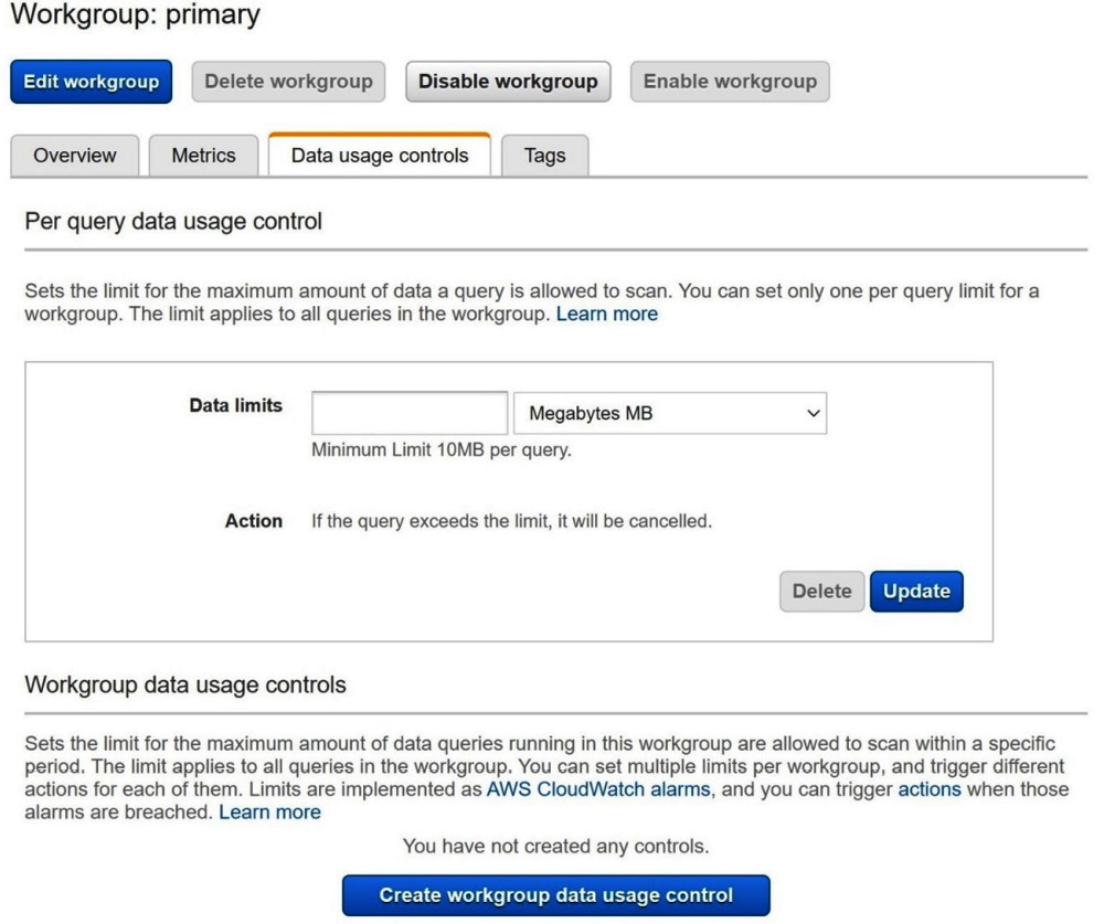
Figure 2.3 – Athena Workgroup settings page; Data usage controls tab

In addition, you can enable CloudWatch metrics for your queries. Once active, Athena will send updated metrics about in-flight and completed queries to CloudWatch, where you can monitor them with your own custom rules, reports, or automation.

Connecting and securing

Connectivity and authentication features are often overlooked. Like all AWS services, Athena offers a set of APIs for interacting with the service from your applications or from the command line when using the AWS CLI. These APIs allow you to submit a new query, check the status of an already running query, retrieve pages of results, or kill a query. These same APIs are used from within Athena's JDBC and ODBC drivers. When connecting to Athena, you can use the standard endpoints if you have an internet gateway in your VPC or opt to call Athena from a VPC endpoint and avoid the need to have internet connectivity from your application VPC. This gives you added control over your security posture by pushing the responsibility of securely connecting to your data sources onto Athena.

In addition to VPC endpoints, Athena also offers SAML federation for managing identities outside of AWS. This allows your Active Directory users to seamlessly authenticate to Athena when using the JDBC or ODBC drivers. At the cornerstone of Athena's access control system lies Lake Formation. Lake Formation allows you to permission IAM users or roles for specific tables, columns, and rows without having to write complex IAM policies to coordinate access to millions of S3 objects or AWS Glue Data Catalog resources.

Now that we've added some basic connectivity options to our performance and cost driver knowledge, we can combine these topics to review common Athena use cases.

Determining when to use Amazon Athena

There is no one answer to this question. There are use cases for which Athena is ideally suited and situations where other tools would be a better choice. Most potential applications of Athena lie in the gradient between these two extremes. This section will describe several common and recommended usages of Athena to help you decide when the right time is for you to use Athena.

Ad hoc analytics

We might as well kick off this discussion with one of Athena's greatest hits – ad hoc analytics. Many customers first notice Athena for its ease of use and flexibility, two key features when you suddenly need to have an unplanned conversation with your data. We saw this firsthand in Chapter 1, Your First Query, when it took us just a few minutes to load up the NYC Taxi trip dataset and start finding relevant business insights. Ad hoc analytics can be used to describe unplanned queries, reports, or research into your data for which a pre-made application, tool, or process does not exist. These use cases often require flexibility, quick iteration times, and ease of use so that a highly specialized skillset is not needed.

For this class of usage, there are relatively few things to consider. The first is where your data is stored. If your data is already in S3 and perhaps already cataloged in AWS Glue, it should be effortless to use Athena as your preferred ad hoc analytics tool. If not, then you will need to think about how you will manage metadata. If your users are savvy, they can create table metadata on the fly using Athena's DDL query language. If not, you may want to consider adding Glue Crawlers to your tool kit. Glue Crawlers automatically scan and catalog data in S3. When complete, the crawlers populate AWS Glue, so you never need to run table create statements manually. Many organizations that are not yet considering or are just starting their data lake journey notice the benefits that come with democratizing access when using Athena for ad hoc analytics. Some organizations go a step further and create a business data catalog. This allows employees to discover datasets and learn their business relevance in addition to the technical details of how and where it is stored. In short, a business data catalog often has more documentation than what is currently offered by the AWS Glue Data Catalog.

Related to the cataloging of data, managing access to that data is another facet to consider. Athena offers two mechanisms for controlling who can read and write analytics data. The first is traditional IAM policies, where you grant individuals or IAM roles access to the specific S3 paths that comprise your tables. This can work well if your data is well organized in S3 and your permission needs are limited to a handful of non-overlapping S3 prefixes. If your needs are more complex, necessitating column or even row-level access control, you'll want to use Athena's Lake Formation integration to manage permissions. In this model, you never have to write IAM policies and instead use an analytics-oriented management console (or APIs) to grant and revoke permissions.

Since ad hoc analytics is a frequent Athena use case, the service has worked with several partners to release driver support in popular BI tools. Tableau and Looker, two popular BI tools, both natively support Amazon Athena. You can also leverage Athena's ODBC and JDBC drivers to query Athena from a slew of other tools, including Microsoft Excel.

The final criteria for using Athena for ad hoc analytics is purely about the kinds of queries you want to run. As we've seen in this chapter, Athena offers limited options for tuning your queries' scale or performance. If your analytics queries often require large amounts of working memory or another extreme scale, you'll want to test how well Athena runs your queries. The good news is that if you eventually encounter a query that Athena struggles with, you can run that outlier with AWS Glue ETL, a serverless form of Spark. That's why it is essential to consider the surrounding ecosystem in addition to Athena's product-specific capabilities. With AWS, the whole is usually greater than the sum of its parts. In Chapter 7, Ad Hoc Analytics, we will get hands-on with more examples of using Athena for this popular recipe.

Adding analytics features to your application

Another popular pattern is to use Amazon to add decision-support information to your application. Imagine we are the authors of a digital advertising campaign system. Our customers use the application to set up new campaigns, monitor the budget of existing campaigns, and even understand the available impression inventory. All this is fancy advertising lingo for understanding different elements of who their campaign is reaching and when they'll exhaust their advertising budget. It would be useful to show some historical trends alongside the current budget remaining number. We can easily use Athena's APIs or JDBC driver to run a query that will return both the hourly impressions, conversions, and budget burndown for the last 24 hours, 7 days, or other relevant timeframes. Because we don't need this data to update live, we can avoid building an OLTP data store. Instead, we need only to feed our existing application logs, or possibly simple metrics, to S3 in a location our Athena queries can access. If we want to be clever, we can even write the metrics to S3 paths based on campaign identifiers and reduce query costs while boosting performance. Thanks to Athena Query Federation, you can go a step further and allow embedded dashboards that show the near-real-time campaign performance only for live campaigns or those within 10% of exhausting their budget. One way to do that is by joining the live status of the campaigns from an OLTP store such as AWS DynamoDB with your historical data from Amazon S3.

We'll go through one more example for good measure. Suppose we are using a machine learning algorithm, such as DeepAR in Amazon SageMaker, to predict demand in our inventory ordering system. The system then automatically reorders ingredients or parts that will be used to replenish our supply of the finished product. For the best results, we've found that the prediction accuracy increased substantially when we supply a week of the most recent sales data as context for the prediction API calls. Unfortunately, our inventory system doesn't keep track of historical inventory burn rates or sales. Well, we could call Amazon Athena to query our data lake's historical order table just before calling our SageMaker prediction endpoint for the next. With a relatively minor enhancement to our application and even less new infrastructure, we've just enabled our inventory system to provide the recent inventory data that will improve our forecasting capabilities.

When considering this usage pattern, you should pay close attention to your anticipated concurrency needs and how the new dependency will affect your application's liveliness. Athena is built for high availability. You don't need to worry about having it in the critical path of your application flow. Still, it's always a good idea to limit critical path dependencies to those that are absolutely necessary. In Chapter 10, Building Applications with Amazon Athena, you will get a chance to see this pattern up close.

Serverless ETL pipeline

With the advent of serverless infrastructure has come a wave of new serverless use cases. Anywhere you previously had a server or cluster of servers running big data jobs has become fair game for Athena's serverless promises. So, it comes as no surprise that customers use Athena to build serverless ETL pipelines. As we stroll toward our imaginary system design whiteboard, let's pretend we work for a hedge fund. Our team is responsible for calculating the company's short risk in response to substantive changes in the stock market. The software that runs our various trading desks generates a file every hour, containing a summary of our long and short positions. Whenever one of these files comes in, we need to recalculate each of the updated stocks' overall positions. Our goal is to ensure that our hedge fund doesn't unknowingly take on too much risk, as was the case with the great Reddit GameStop uprising of 2021.

GameStop won't stop

The saga of GameStop, GME, began in August 2020 when an anonymous user on Reddit posted an in-depth analysis and justification for why GameStop would go to the moon. In addition to a few solid fundamental theories, this person highlighted the absurd reality that GameStop shares had a short interest greater than 100% of the available shares. This means that for every share of GameStop stock, more than one share had been sold. This happens when people, or companies, bet against the stock by borrowing shares from their broker and sell them to someone else. You are said to be short with the stock because you now owe someone else a share you borrowed. What began as a way to make money sticking to the shorts morphed into a socio-economic movement pitting the underdog retail investor against some of the biggest hedge funds in the world. No matter which side you were on, it was unprecedented. It also generated many amusing memes.

Using Athena and AWS Lambda, a serverless technology for responding to events, we can configure S3 to send an event to Lambda whenever a new trade summary file arrives in our S3 bucket. When the file comes, a Lambda function gets invoked. Within that function, we can run custom code to have Athena query the newly added file and join it with relevant information from a dimension table before writing the results to our data lake in Parquet format. After the initial transform and load, we trigger another Lambda function, which reruns our overall risk analysis Athena query to determine whether we are overexposed to one or more securities. Without touching a single server, we built an entire ETL pipeline, albeit a relatively simple one. Depending on the data sizes involved, it's not unreasonable for this ETL pipeline to cost mere pennies a day.

While simple ETL pipelines can be appropriate for Athena, you should consider the number and size of jobs you expect to run in your ETL system. Like earlier examples, the AWS ecosystem has complementary capabilities in AWS EMR and AWS Glue ETL, which can help if you outgrow or run into requirements that Athena cannot satisfy. AWS Glue ETL is also serverless, though it is based on Apache Spark and charges you for compute time instead of Athena's Presto-based engine, which charges by the terabyte scanned. In Chapter 9, Serverless ETL Pipelines, we will go step by step and build out a reactive ETL pipeline.

We will conclude our review of common Athena use cases by discussing a few miscellaneous examples that, while too small to dedicate a full section to, are equally valid.

Other use cases

While less prominent than the use cases described in previous sections, some customers use Athena as an operational tool or a rapid prototyping tool. Athena's filtering performance makes it a rather performant choice for rapidly scaling and filtering log data without the need to keep a costly infrastructure running all the time. This is ideal for operation situations that arise from nowhere. Customers filter and parse everything from VPC flow logs to application logs, looking for root causes or quantifying impact. Athena's flexibility also makes it a great choice to quickly iterate on complex reports or ETL jobs that you'll later implement in a different system. This is not unlike other data preparation use cases from machine learning or data quality checking.

Just because a use case you have in mind wasn't explicitly mentioned in this chapter doesn't mean you should consider Athena. We've only listed examples of good use cases so that you can extrapolate and apply what you've learned to your projects and environment.

Summary

In this chapter, we formalized your introduction to Athena by going over the service's high-level capabilities, including ACID transactions, federation, ETL operations such as CTAS, and open source file formats. We went inside Athena by learning more about Presto, the open source distributed SQL engine that sits at its core. As part of that exercise, we experimented with supporting our own multi-tenant analytics infrastructure. This allowed us to see all the value-added functionality that sets Athena apart from other serverless technologies that fall short of being fully managed. As if that wasn't enough of a reason to hop on the serverless analytics bandwagon, we unpacked the marketing hype to find that Athena's $5/TB price tag is significantly cheaper than many of its competitors who also claim to charge $5/TB, but count the uncompressed bytes!

We also learned that performance is personal and that we'd have to test our access patterns and data models to see how Athena would perform for us. Regardless of the numerous variables that impact performance, we covered how to control common cost and performance drivers by using columnar storage formats such as Apache Parquet. Using these techniques dramatically reduces our costs but subtly increases the additional costs associated with the other services Athena calls on our behalf, including S3, AWS Glue, and AWS KMS. In addition to pre-emptive actions to control costs, Athena also gave us mechanisms to limit the total cost of each query or group of queries through workgroup-level limits on data scans.

Lastly, we combined all these points when reviewing several common usage patterns for Athena. We walked through a real-world example using a hypothetical system design for each of the frequently seen patterns. We'll be revisiting each of these design patterns in later chapters, where we will get hands-on and build one of each.

The next chapter will conclude our introduction to Amazon Athena by exploring built-in features you can use to make your reports or application more powerful. This includes approximate query techniques to speed up analysis of large datasets, CTAS (CREATE TABLE AS SELECT) statements for running queries that generate significant amounts of result data, and getting hands-on with several of the topics discussed in this chapter.

Further reading

In this section, we've gathered links to additional materials that you may find useful in diving deeper into some of the primary sources regarding the topics mentioned in this chapter. Many of these topics will be covered in more detail later in this book, but it can often be useful to know where to go for authoritative details:

• Presto SQL Dialect documentation can be found here: http://bit.ly/39kMJeW.
• Amazon Athena SQL Dialect documentation can be found here: http://amzn.to/35tRT7w.
• Amazon leadership principles can be found here: http://bit.ly/3k79PuB.
• Amazon Athena Engine Version 1 specification can be found here: http://bit.ly/3boEoty.
• Amazon Athena Datasource and External Hive Metastore documentation can be found here: http://amzn.to/3bvU9y.
• The official GDPR regulation and associated data retention requirements discussed in this chapter can be found here: http://bit.ly/38RlolU.
• Details for connecting Athena to Delta Lake from SymlinkTextInputFormat can be found in the Delta Lake documentation here: http://bit.ly/3ozT9gG.
• More information about the TPC organization and the industry benchmarks it maintains (TPCH/DS) can be found here: http://bit.ly/39HMXgJ.
• You can find the Athena Federation SDK on GitHub here: http://bit.ly/38NfRg4.
• Trino, formerly PrestoSQL, documentation can be found here: http://bit.ly/39JLGFE.
• The original Presto white paper from Facebook can be found here: https://bit.ly/38vQgI8.