Search in book...
Toggle Font Controls
Create new playlist

Name your new playlist

Playlist description (optional)
Sign In

Email address

Password

Forgot Password?

or

Continue with Facebook

Continue with Google
Sign Up

Full Name

Email address

Confirm Email Address

Password

or

Continue with Facebook

Continue with Google

Chapter 8: Querying Unstructured and Semi-Structured Data

Many of the world's most valuable datasets are loosely structured. They come from application logs, which don't conform to any standards. They come from event data generated by a system that users interact with, such as a web server, which stores how users navigate an organization's website. They can also come from an analyst generating spreadsheets on a company's financial performance. This data is usually stored and shared in a semi-structured format to make it easier for others to consume. Some query engines have evolved to fully support this semi-structured data.

When talking about structured, semi-structured, and unstructured data, there are many different definitions out there. For this book, structured data is stored in a specialized data format where the schema and the data it represents are one to one. The data is serialized to optimize how the data is read, written, and analyzed. An example is a relational database. Semi-structured data is when the data format follows a specific format, and a schema can be provided to read that data. For example, the JSON, XML, and CSV file formats have rules on how they are parsed and interpreted. Still, the relationship to a schema or table definition is loose. Unstructured data is data that does not follow a particular data model. Examples of unstructured data include application logs, images, text documents, and more.

In this chapter, we will learn how Amazon Athena combines a traditional query engine and its requirement for an up-front schema with extensions that allow it to handle data that contains varying schemas or no schema at all.

In this chapter, we will cover the following topics:

Why isn't all data structured to begin with?
Querying JSON data
Querying arbitrary log data

Technical requirements

For this chapter, if you wish to follow some of the walk-throughs, you will require the following:

Internet access to GitHub, S3, and the AWS Console.
A computer with Chrome, Safari, or Microsoft Edge installed.
An AWS account and an accompanying IAM user (or role) with sufficient privileges to complete this chapter's activities. For simplicity, you can always run through these exercises with a user who has full access. However, we recommend using scoped-down IAM policies to avoid making costly mistakes and learn how to best use IAM to secure your applications and data. You can find a minimally scoped IAM policy for this chapter in the book's accompanying GitHub repository, listed as chapter_8/iam_policy_chapter_8.json (https://bit.ly/3hgOdfG). This policy includes the following:
- Permissions to create and list IAM roles and policies:
  - You will be creating a service role for an AWS Glue Crawler to assume.
- Permissions to read, list, and write access to an S3 bucket.
- Permissions to read and write access to Glue Data Catalog databases, tables, and partitions:
  - You will be creating databases, tables, and partitions manually and with Glue Crawlers.
- Access to run Athena queries.

Why isn't all data structured to begin with?

Data is generated from everywhere at all times within computer systems. They power our applications and reports and help us make sense of the world and our decisions that impact it. Data that's produced from an application that manages financial portfolios tells us how much risk the instruments in the portfolio are at. Websites can generate click data to tell a story, such as how customer's behavior changes when an update is made to a website. Retail businesses produce sales transactions and marketing data to determine how sales are affected by marketing campaigns. Amazon's user traffic information on individual products can train machine learning models to make recommendations to users who showcase products that they didn't even know they wanted. For this data to be helpful, it must be accessible to data engineers and machine scientists to produce even greater value from them.

However, not all data is created equally. If we take a hypothetical online store that sells everything from A to Z, sales information can be saved in structured data stores such as relational databases. User traffic and click data can be stored as text files in S3 in CSV files. Item description data can be retrieved through a RESTful API and saved as JSON data. The format and structure of the data are usually chosen based on how best to represent the information and how downstream applications consume that information. Usually, this data is not stored in a database system because this tends to be expensive. Hence, they are pruned of older data to keep costs low and performance high. Having data in a semi-structured format makes sharing data very easy. The data usually conforms to open standards, such as CSV, JSON, and XML. It is also estimated that 80-90% of current applications produce non-structured data. So, it makes sense to not change the existing applications but have our query engine read the data directly or ETL the data for Athena to read.

The remainder of this chapter will show you how to query a variety of semi-structured and unstructured data sources using Athena. We will use a fictitious retail business that sells widgets. This retail business wants to perform analytics with data that is produced by various systems. The following table outlines the system and type of data that is generated:

Table 8.1 – Data types and descriptions

The sample data files can be found on GitHub (https://bit.ly/3wlJSwV). Let's query these datasets.

Querying JSON data

JSON is a prevalent data format. It can be described as a lightweight version of XML and has many similarities with it. The file format is text-based, contains field names, along with their values, and supports advanced data types such as structures and arrays. A structured data type is a group of columns that are stored and referred to by their structure names and column names. This allows for logically similar columns to be grouped; for example, the structure of a customer's address that contains a street name, street number, city, state, and more. Arrays allow a single row to have a field containing zero or more values that can be referenced by an index number. An example list would be a list of addresses for a customer. JSON supports a mixture of arrays and structures. You can have an array of structures or a structure with an array field within it.

When using Athena, JSON files have to be of a particular format. Athena requires that JSON files must contain a single JSON object on separate lines within a file. If there are multiple objects on the same line, only the first object will be read, and if an object spans multiple lines, it will not throw an error. If the file format does not conform to what is compatible with Athena, then the data will need to be transformed (see Chapter 9, Serverless ETL Pipelines ).

Now, let's look at some sample queries and read our customer's table.

Reading our customer's dataset

The following is a sample JSON record from our customer's table (formatted to be easier for a human to read but not Athena!):

{

"customer_id": 10,

"first_name": "Mert",

"last_name": "Hocanin",

"email": "[email protected]",

"addresses": [

{

"address": "63 Fairview Alley",

"city": "Syracuse",

"state": "NY",

"country": "United States"

}

]

}

Here, we can see that this record has five fields: customer_id, first_name, last_name, email, and addresses. The addresses field is an array that contains a structure that contains four fields.

To register this table in our catalog, we can run a Glue crawler. But if we want to create this table using a CREATE TABLE statement (available at https://bit.ly/3yna5eV), it would look like this:

CREATE EXTERNAL TABLE customers (

customer_id INT,

first_name STRING,

last_name STRING,

email STRING,

addresses ARRAY<STRUCT<address:STRING,city:STRING,state:STRING,country:STRING>>,

extrainfo STRING

)

ROW FORMAT SERDE

'org.openx.data.jsonserde.JsonSerDe'

STORED AS INPUTFORMAT

'org.apache.hadoop.mapred.TextInputFormat'

OUTPUTFORMAT

'org.apache.hadoop.hive.ql.io.HiveIgnoreKeyTextOutputFormat'

LOCATION

's3://<S3_BUCKET>/chapter_8/customers/';

Let's view some sample data from this table by running SELECT * FROM customers LIMIT 10:

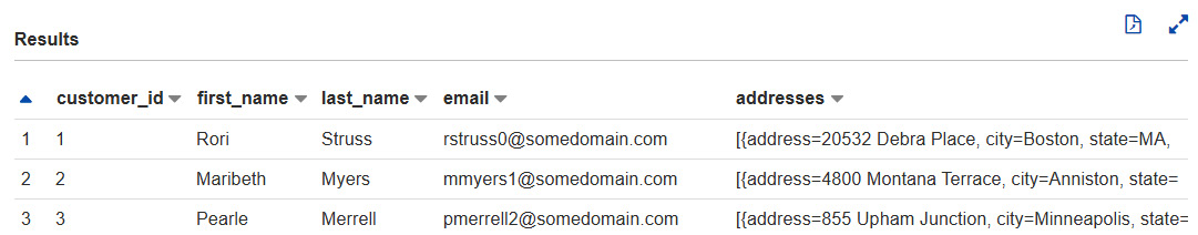
Figure 8.1 – Sample data from the customers table

The results look as expected. Now, let's query the table and see how many customers have primary addresses in each state. We will assume that the first address in the address list is their primary address, so we can run the following query:

SELECT

addresses[1].state AS State,

count(*) AS Count

FROM customers

WHERE cardinality(addresses) > 0

GROUP BY 1 ORDER BY 2 DESC LIMIT 5

The results will look as follows:

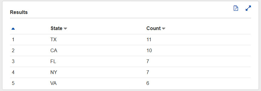
Figure 8.2 – Query results to show the top five numbers of customers by US state

With arrays, we can reference the element by using square brackets (addresses[1]). Since this returns a structure, we can reference the field by its name (.state). So, putting this together, we can specify the first address's state by writing addresses[1].state. Now, let's look at how we can parse fields that contain JSON data.

Parsing JSON fields

There are cases where some fields contain a string that contains JSON as a payload. This is sometimes done to make the payload completely abstract. Only the readers of the payload would understand the data in it. Our customer's table has a field called extrainfo containing JSON. In this section, we will describe an unlimited shipping program called the Pinnacle program. When we run SELECT customer_id, extrainfo FROM customers WHERE extrainfo is not null LIMIT 5, we get the following results:

Figure 8.3 – The extrainfo field within the customers table

So, what can we do with this JSON data in the field? Athena (and PrestoDB/TrinoSQL) supports a JSON data type and a variety of built-in functions that allow us to interact with the JSON data easily without parsing or transforming the data. There are two JSON functions that are really useful: json_extract and json_extract_scalar. These functions take a string and a JSON path and return the JSON data type or a string. These functions extract any field within the JSON object, regardless of how nested the data may be. For example, if we run SELECT json_extract_scalar(extrainfo, '$.is_pinnacle_customer') FROM customers where extrainfo IS NOT NULL , we would get the following result:

Figure 8.4 – json_extract_scalar function example

Let's look at some things we should consider when reading JSON data.

Querying comma-separated value and tab-separated value data

The comma-separated value (CSV) and tab-separated value (TSV) formats are some of the oldest data formats. They have lasted the test of time. They are heavily used today in many legacy systems and even among heavy Microsoft Excel users. Their main advantages versus other formats are their simplicity, their popularity, and that most spreadsheet applications can open them. CSV and TSV data also map very closely to tables within a database, where you have rows and columns of data. CSV and TSV files are text-based. Field values are separated by a delimiter, usually commas or tabs, and rows are separated by newlines. You can find examples of CSV files at https://bit.ly/2TQY8z5 and https://bit.ly/3h1G919. We will use them as example datasets. Let's look at an example.

Reading a typical CSV dataset

Reading CSV and TSV data within Athena is simple, and in most cases, it is very straightforward. For most use cases, we can use the built-in delimited text parser. Let's take a look at the CREATE statement for our sales table (this can be found at https://bit.ly/2TQG73W):

CREATE EXTERNAL TABLE sales (

timestamp STRING,

item_id STRING,

customr_id INT,

price DOUBLE,

shipping_price DOUBLE,

discount_code STRING

)

ROW FORMAT DELIMITED

FIELDS TERMINATED BY ','

ESCAPED BY ''

LINES TERMINATED BY ' '

LOCATION 's3:// <S3_BUCKET>/chapter_8/sales/'

TBLPROPERTIES ('serialization.null.format'='',

'skip.header.line.count'='1')

We can set two table properties here: skip.header.line.count and serialization.null.format. The skip.header.line.count property tells the parser to skip the first line in the CSV file as it contains the column names or the header row. The serialization.null.format property tells the parser to treat empty columns as nulls. Now that we have defined our sales data, let's take a look at some sample data, as shown in the following screenshot:

Figure 8.5 – Sample data from the sales dataset

If your data contains a string field containing a comma, you can deal with it in two ways. First, you can escape the comma by using the specified character provided by the ESCAPED BY value. The second would be to surround the field with quotes, but you will need to use the OpenCSVSerDe parser for Athena to parse quoted fields correctly. We'll look at OpenCSVSerDe in more detail later. Now, let's learn how to read TSV files.

Reading a typical TSV dataset

TSV files are similar to CSV files, except tabs are used as delimiters between field values rather than commas. Tabs are less likely to be contained within string fields, so they are sometimes convenient to use rather than commas and escape unintentional commas. If you have tried to open a CSV file with Microsoft Excel and the columns do not align with these unexpected commas, you will understand that they can be challenging to fix.

In our example, we have a table representing marketing campaigns that contains a starting timestamp that represents the start of a marketing campaign, an ending timestamp that represents the end of a marketing campaign, and a description of the campaign. Suppose the marketing department provides this data as an export from Microsoft Excel that delimited the fields by tabs. To register the table, the CREATE TABLE statement (available at https://bit.ly/3xZVIwU) will look very similar to the CSV table, as shown in the following statement:

CREATE EXTERNAL TABLE marketing (

start_date STRING,

end_date STRING,

marketing_id STRING,

description STRING

)

ROW FORMAT DELIMITED

FIELDS TERMINATED BY ' '

ESCAPED BY ''

LINES TERMINATED BY ' '

LOCATION 's3:// <S3_BUCKET>/chapter_8/marketing/';

You'll notice that the delimiter is , which represents a tab. The sample data is shown in the following screenshot:

Figure 8.6 – Sample data from the marketing dataset

You will notice a comma in the second row that we did not need to escape. Now that we have a dataset for sales, customers, and marketing information, we can do some simple analytics from data that could have come from three different systems or sources. Let's look at a quick example.

Example analytics query

Suppose that we wanted to know how effective our marketing campaigns were by looking at the number of sales on days with campaigns versus days that do not. Additionally, we want to know the states that the sales were coming from. The following is a sample analytics function that can achieve that (this can be found at https://bit.ly/3gXwf1u, which also contains a breakdown of the query):

SELECT

date_trunc('day', from_iso8601_timestamp(sales.timestamp)) as sales_date,

CASE WHEN marketing.marketing_id is not null then TRUE else FALSE END as has_marketing_campaign,

SUM(1) as number_of_sales,

histogram(CASE WHEN cardinality(customers.addresses) > 0 THEN customers.addresses[1].state ELSE NULL END) as states

FROM

sales

LEFT OUTER JOIN

marketing

date_trunc('day', from_iso8601_timestamp(marketing.start_date))

= date_trunc('day', from_iso8601_timestamp(sales.timestamp))

LEFT OUTER JOIN

customers

sales.customer_id = customers.customer_id

GROUP BY 1, 2 ORDER BY 3 DESC

This Athena query would produce the following results:

Figure 8.7 – Results of the analytics query

Here, we can see that for our top three results, days that had marketing campaigns produced the most sales and that most of our sales came from California. This information can help inform future marketing campaigns as well as inventory when marketing campaigns are run. This was just a warmup; we will look at more cases and explain how to do this type of analytics in Chapter 7, Ad Hoc Analytics. Now, let's learn how to read inventory data.

Reading CSV and TSV using OpenCSVSerDe

So far, we have looked at using the default version of SerDe to parse CSV and TSV files. However, another SerDe that we should look at deals with CSV and TSV files called OpenCSVSerDe. This SerDe compares to the default SerDe in a few crucial ways. First, it supports quoted fields, meaning that values are surrounded by quotes. This is usually done when the fields contain the same delimiter values, which are then ignored until the quote values are found. However, if there are quote values, those need to be escaped as well. The second difference is that all columns are treated as STRING data types, regardless of the table definition, and need to be implicitly or explicitly converted into the actual data type. The following is a sample CSV file from our inventory dataset that illustrates when OpenCSVSerDe should be used:

"inventory_id","item_name","available_count"

"1","A simple widget","5"

"2","A more advanced widget","10"

"3","The most advanced widget","1"

"4","A premium widget","0"

"5","A gold plated widget","9"

If we used the default SerDe, the inventory_id and available_count data would need to be specified as a string, and all field values would be returned with quotes, as shown in the following screenshot:

Figure 8.8 – Reading the inventory dataset using the default SerDe

When the data is returned, as shown in the preceding screenshot, it would be tough to use. Using OpenCSVSerDe will solve this issue, as shown in the following CREATE TABLE statement (which is available at https://bit.ly/35UsP9k):

CREATE EXTERNAL TABLE inventory (

inventory_id BIGINT,

item_name STRING,

available_count BIGINT

)

ROW FORMAT SERDE 'org.apache.hadoop.hive.serde2.OpenCSVSerde'

WITH SERDEPROPERTIES ("separatorChar" = ",", "escapeChar" = "\")

LOCATION 's3://<S3_BUCKET>/chapter_8/inventory/'

TBLPROPERTIES ('skip.header.line.count'='1')

Using OpenCSVSerDe will give us the following results:

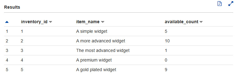
Figure 8.9 – Inventory data using OpenCSVSerDe

For more information about using OpenCSVSerDe, see Athena's documentation, which is located at https://amzn.to/3isnvzr.

Now that we have learned how to read CSV and TSV data that's been generated from Microsoft Excel or another source, let's dive into reading arbitrary log data.

Querying arbitrary log data

One very common use case for system engineers or software developers is to scan log files to find a particular logline. This may be to find when bugs have occurred, gather metrics about how a specific system performs, how users interact with a system, or to diagnose user or customer issues. There is a vast amount of useful and valuable data that comes out of log data. It's a great idea to store application log data in data to be mined in the future. Many of the AWS services are already pushing log data into S3 or can easily be configured. Athena's documentation provides templates for reading many of these services' log files, which can be found at https://amzn.to/3dJzt6H. Let's learn how Athena can be used to quickly and easily scan through logs stored on S3.

Doing full log scans on S3

Many logs are pushed to S3. Reading through those log files can be difficult and/or time-consuming when stored on S3. If those logs need to be read to look for problems, issues, or some kind of event, you may download the files and then run a grep command. This could take a lot of time because the download from S3 is done using a single computer, so it is limited by a single computer's network and CPU resources. You could spin up a Hadoop cluster and attempt to read the logs in parallel, but that requires expertise in using Hadoop and the time it takes to create and configure the cluster.

Athena can scan your log files in a parallel and easy way and return lines in log files that match search criteria. Let's go through an example. Anyone who has used Amazon EMR before knows that the application logs of Apache Hive, Apache Spark, and other applications are pushed to S3. When a particular Spark or Hive job fails, finding the specific log file that caused the failure may be difficult. Using Athena, we can search for the failure and log out the files that contained those failures. To do this scanning, we will rely on the default version of SerDe that Athena provides, which we looked at in the Querying comma-separated value and tab-separated value data section. But the trick here is to specify a delimiter that is very unlikely to exist in our log files. Let's look at CREATE TABLE:

CREATE EXTERNAL TABLE emrlogs (

log_line string

)

ROW FORMAT DELIMITED

FIELDS TERMINATED BY '|'

LINES TERMINATED BY ' '

LOCATION

's3://<S3_BUCKET>/elasticmapreduce/j-2ABCDE34F5GH6'

Since the pipe character is unlikely to be in EMR logs, the log_line field will contain the value of a single logline. Then, we can submit queries while looking for a specific text. For example, we can use regexp_like to specify a regex to search for:

SELECT log_line FROM emrlogs where regexp_like(log_line, 'ERROR|Exception')

This query will print the entire line. Although this can be useful, we can also specify a hidden column that gives us the path of the file that the row was found in:

SELECT log_line, "$PATH" FROM emrlogs where regexp_like(log_line, 'ERROR|Exception')

The $PATH field is very useful as it will give us the path that the logline was found in to download the file or files and take a closer look. The $PATH field can also be put in the WHERE clause to search for a particular application, EC2 instance ID, or EMR step ID. The following screenshot shows the example query output from the previous query:

Figure 8.10 – Running a Grep search on EMR logs using Athena

This way of using Athena can be applied to any text-based log files and can make it quick and easy to scan logs stored on S3. But what if we wanted to scan log files that are a little more structured to filter based on fields? This is where using Regex and Grok SerDes can help.

Reading application log data

Athena has two built-in SerDes that allow you to parse log data that follows a pattern. They then map the pattern to different columns within a table to query many types of log files. These two SerDes are the Regex SerDe and the Grok SerDe. With both of these SerDes, you provide an expression that Athena will use to parse each line of your text file and map the expressions to columns in your table.

Regular expressions, or regexes for short, are commonly used within many programming languages and editors to provide a search expression to find or replace a particular pattern. We won't go into how to write regular expressions, but if you are familiar with how to write regular expressions, then the Regex SerDe can be useful. The good news is that for many types of application logs, Athena's documentation provides the expressions so that they're ready to use to parse some of the most popular log types, such as Apache web server logs (see https://amzn.to/3xqrNhO) and most AWS services (see https://amzn.to/3dJzt6H). If you do want to create regular expressions for other log types, then we recommend using an online regular expression evaluator to test your expressions, which can help.

The Grok SerDe was built based on Logstash's grok filter. This SerDe takes in a Grok expression that is used to parse log lines. Grok expressions can be seen as extensions of regexes as Grok expressions are built using regexes, but regex expressions can be named and referenced. With named expressions, you can put them together to express a full logline in a more human-readable format. An added benefit is that Logstash has many built-in, ready-made expressions that you can use. The list is available at https://bit.ly/3hEqq8n. Let's look at an example of how this works.

Let's take our fictional company. They have a web server that outputs when visits occur, which page they visited, and referred them. Some example rows are as follows:

1621880197 59.73.211.164 http://www.acmestore.com/ https://www.yahoo.com

1597343145 50.13.226.237 http://www.acmestore.com/ https://www.google.com

1617872146 32.2.141.225 http://www.acmestore.com/product/4 https://www.duckduckgo.com

1621960907 65.105.235.14 http://www.acmestore.com/product/1 https://www.google.com

We have the time in epoch format, the visitor's IP address, the page that was visited, and the referrer (usually a search engine). Looking at the pre-built grok expressions, the preceding code can be expressed as "%{NUMBER:time_epoch} %{IP:source_addr} %{URI:page_visited} %{URI:referrer}?". Let's create the table and query it using the following CREATE TABLE (available at https://bit.ly/3xjRxMD):

create external table website_clicks (

time_epoch BIGINT,

source_addr STRING,

page_visited STRING,

referrer STRING

) ROW FORMAT SERDE

'com.amazonaws.glue.serde.GrokSerDe'

WITH SERDEPROPERTIES (

'input.format'='%{NUMBER:time_epoch} %{IP:source_addr} %{URI:page_visited} %{URI:referrer}?'

)

STORED AS INPUTFORMAT

'org.apache.hadoop.mapred.TextInputFormat'

OUTPUTFORMAT

'org.apache.hadoop.hive.ql.io.HiveIgnoreKeyTextOutputFormat'

LOCATION

's3:// <S3_BUCKET>/chapter_8/clickstream/';

The SerDe we specified is com.amazonaws.glue.serde.GrokSerDe, and we put it in the Grok expression via the input.format SerDe property. Now, if we query the table, we will get the following results:

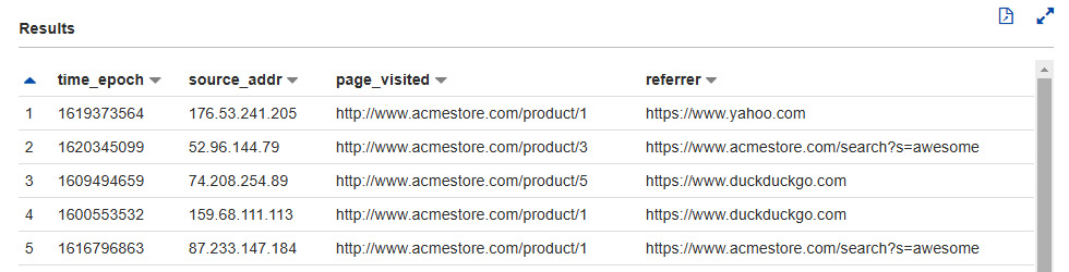
Figure 8.11 – Running a query against a table using Grok SerDe

Now that we can parse and query application logs, let's summarize what we have learned so far.

Summary

In this chapter, we explored the different ways in which we can query unstructured and semi-structured data. This data that comes from applications, databases, or even Microsoft Excel can be queried using Athena. We looked at two of the most commonly used file formats used by legacy and source systems, JSON and CSV/TSV, and how to determine which SerDes to use to parse them. We then looked at the Regex and Grok SerDes to help us parse log files that conform to some patterns, such as Log4J logs. Using these SerDes, we can query and derive value.

The next chapter will examine how we can take unstructured and semi-structured data and transform it into a more performant and cost-effective format, such as Apache Parquet or Apache ORC.

Table of Contents for
Chapter 8: Querying Unstructured and Semi-Structured Data

Chapter 8: Querying Unstructured and Semi-Structured Data

Technical requirements

Why isn't all data structured to begin with?

Querying JSON data

Reading our customer's dataset

Parsing JSON fields

Other considerations when reading JSON

Schema updates with JSON

JSON SerDe comparison