
Chapter 3: Key Features, Query Types, and Functions
In Chapter 1, Your First Query, we got our first taste of serverless analytics by building and querying a mini-data lake for New York City (NYC) taxicab data. Chapter 2, Introduction to Amazon Athena, continued that introduction by helping us understand and perhaps appreciate what goes into enabling Athena's easy-to-use experience. This chapter will conclude our introduction to Amazon Athena by exploring built-in features you can use to make your reports or applications more powerful. Unlike the previous chapter, we will return to a hands-on approach that combines descriptive instruction with step-by-step activities that will help you connect with the material. The exercises should also offer you a basis to experiment with your own ideas, should you choose to do so.
After completing this chapter, you will have enough knowledge to begin using and integrating Athena into proof-of-concept (POC) applications. Chapter 4, Metastores, Data Sources, and Data Lakes, begins Part Two of this book, which transitions to broader topics associated with building and connecting your data lake as part of delivering sophisticated analytics strategies and applications at scale.
In the subsequent sections of this chapter, you will learn about the following topics:
- Running extract-transform-load (ETL) queries
- Running approximate queries
- Organizing workloads with WorkGroups and saved queries
- Using Athena's application programming interfaces (APIs)
Technical requirements
Wherever possible, we will provide samples or instructions to guide you through the setup. However, to complete the activities in this chapter, you will need to ensure you have the following prerequisites available. Our command-line examples will be executed using Ubuntu, but most Linux flavors should work without modification, including Ubuntu on Windows Subsystem for Linux (WSL).
You will need internet access to GitHub, Simple Storage Service (S3), and the Amazon Web Services (AWS) console.
You will also require a computer with the following installed:
- The Chrome, Safari, or Microsoft Edge browsers
- The AWS Command-Line Interface (CLI)
This chapter also requires you to have an AWS account and an accompanying Identity and Access Management (IAM) user (or role) with sufficient privileges to complete this chapter's activities. Throughout this book, we will provide detailed IAM policies that attempt to honor the age-old best practice of least privilege. For simplicity, you can always run through these exercises with a user that has full access. Still, we recommend using scoped-down IAM policies to avoid making costly mistakes and we advise you to learn more about using IAM to secure your applications and data.
You can find the suggested IAM policy for this chapter in the book's accompanying GitHub repository listed as chapter_3/iam_policy_chapter_3.json, here: http://bit.ly/37zLh8N. The primary changes from the IAM policy recommended for Chapter 1, Your First Query, include the following:
- glue:BatchCreatePartition—Used to create new partitions as part of CTAS or INSERT INTO statements.
- Restricted Athena workgroup actions to WorkGroups beginning with packt-*.
- Added read/write access for AWS CloudShell, a free Linux command line in the AWS console. You only pay for the other services you interact with, such as Athena.
Running ETL queries
While this book's goal is not to teach Structured Query Language (SQL), it is beneficial to spend some time reviewing everyday SQL recipes and how they relate to Athena's strengths and quirks. Transforming data from one format to another, producing intermediate datasets, or simply running a query that outputs many megabytes (MB) or gigabytes (GB) of output necessitates some understanding of Athena's best practices to achieve peak price/performance. As we did in Chapter 1, Your First Query, let's start by preparing a larger dataset for our exercises.
We will continue using the NYC Yellow Taxi dataset, but we will prepare 2.5 years of this data this time. Preparing this expanded dataset will entail downloading, compressing, and then uploading dozens of files to S3. To expedite that process, you can use the following script to automate the steps. To do so, add all the files from yellow_tripdata_2018-01.csv through yellow_tripdata_2020-06.csv. Each file represents 1 month of data. The NYC Taxi and Limousine Commission has not updated the data since June 2020 due to the impact the pandemic has had on their day-to-day operations. If you have the option, we recommend downloading a copy of the pre-made script with added error checking from the book's companion GitHub repository in the chapter_3/taxi_data_prep.sh file or by using this link: http://bit.ly/3k4bMYU. The following script has been edited for brevity, but the one in GitHub is ready to go without modification. Regardless of which script you use, you can run it on any Linux system with wget and the AWS CLI installed and configured by executing it and passing the name of the S3 bucket where you'd like the data uploaded. You can even reuse the S3 bucket we created in Chapter 1, Your First Query, to save time.
AWS CLI
The taxi_data_prep.sh script will use your system's AWS CLI to upload the compressed taxicab data to the S3 bucket you specify. The script expects you to have configured the AWS CLI ahead of time with appropriate credentials and a default region that corresponds to where you are running the exercises in this book. To review or update your default AWS CLI configuration, you can run aws configure at the command line.
The configuration is shown here:
#!/bin/bash
BUCKET=$1
array=( yellow_tripdata_2018-01.csv
yellow_tripdata_2018-02.csv
# some entries omitted for brevity
yellow_tripdata_2020-06.csv
)
for i in "${array[@]}"
do
FILE=$i
ZIP_FILE="${FILE}.gz"
wget https://s3.amazonaws.com/nyc-tlc/trip+data/${FILE}
gzip ${FILE}
aws s3 cp ./${ZIP_FILE} s3://$BUCKET/chapter_3/tables/nyc_taxi_csv/
rm $ZIP_FILE
done
Code 3.1 – NYC taxi data preparation script
Speeding things up!
Depending on the speed of your internet connection and the type of central processing unit (CPU) you have, this script may take over an hour to prepare the 4.5 GB of data for the recommended 2.5 years of historical data. We recommend using AWS CloudShell (https://aws.amazon.com/cloudshell/) to run this script natively within the AWS ecosystem. AWS CloudShell provides a Linux command line with AWS CLI and other common tools preinstalled at no extra charge. You are only charged for the other services you interact with, not for your usage of CloudShell itself. In our testing, AWS CloudShell took roughly 23 minutes to prepare our test data, thanks in part to its high-speed connectivity to Amazon S3. Alternatively, you can reduce the amount of historical data you use in the exercise by reducing the number of monthly files used in the script.
Once the script completes execution, you can verify your data is now in the proper location by listing S3 from the command line using the following command or navigating to /chapter_3/tables/nyc_taxi_csv/ from the S3 console in your browser. If all went well, you'd see 30 files in this path:
aws s3 ls s3://YOUR_BUCKET_NAME_HERE/chapter_3/tables/nyc_taxi_csv/
Our final data preparation step is to use Athena to define a table rooted at the path we uploaded the data to. To do this, we'll apply our final Chapter 1, Your First Query, refresher in the form of a CREATE TABLE query. If you have the option, we recommend downloading a copy of the following CREATE TABLE query from the book's companion GitHub repository in the chapter_3/create_taxi_table.sql file or by going to https://bit.ly/2TOinOs:
CREATE EXTERNAL TABLE 'packt_serverless_analytics'.'chapter_3_nyc_taxi_csv'(
'vendorid' bigint,
'tpep_pickup_datetime' string,
'tpep_dropoff_datetime' string,
'passenger_count' bigint,
'trip_distance' double,
'ratecodeid' bigint,
'store_and_fwd_flag' string,
'pulocationid' bigint,
'dolocationid' bigint,
'payment_type' bigint,
'fare_amount' double,
'extra' double,
'mta_tax' double,
'tip_amount' double,
'tolls_amount' double,
'improvement_surcharge' double,
'total_amount' double,
'congestion_surcharge' double)
ROW FORMAT DELIMITED
FIELDS TERMINATED BY ','
STORED AS INPUTFORMAT
'org.apache.hadoop.mapred.TextInputFormat'
OUTPUTFORMAT
'org.apache.hadoop.hive.ql.io.HiveIgnoreKeyTextOutputFormat'
LOCATION
's3://<YOUR_BUCKET_NAME>/chapter_3/tables/nyc_taxi_csv/'
TBLPROPERTIES (
'areColumnsQuoted'='false',
'columnsOrdered'='true',
'compressionType'='gzip',
'delimiter'=',',
'skip.header.line.count'='1',
'typeOfData'='file')
Code 3.2 – CREATE TABLE SQL query
You can execute this query right from the Athena console, but be sure to update the S3 bucket in the LOCATION portion of the CREATE TABLE statement. The table creation should complete almost instantaneously. The most common errors at this stage are related to insufficient permissions, using an incorrect database or table name, or already having a table with that name in your catalog. In the event you do encounter an issue, retrace your steps, and double-check these items. It's always a good practice to run at least one query to ensure our table is properly set up since the CREATE TABLE operation is purely a metadata operation. That means it didn't actually list or read any of the data we prepared in S3. A simple COUNT(*) query, as illustrated in the following code snippet, will suffice to ensure our table is ready to be used in more ambitious queries:
select count(*) from chapter_3_nyc_taxi_csv
After running the preceding query from the Athena console, you should get a result of 204,051,059. The query should have scanned around 3.4 GB of data and completed after roughly 8 seconds. We have just completed one of the most common activities you'll encounter in Athena or any data lake analytics tool. The table we just created is commonly described as a landing zone. It is a place where newly arrived source data lands before being cleaned up and made available to applications in your data lake. Data ingestion is always where it begins, but the table we just created is sub-optimal for a number of reasons, and we may not want to let applications or analysts use it directly. Instead, we will reorganize this table for peak performance as a way to demonstrate some of Athena's advanced query types, such as CTAS, INSERT INTO, and TABLESAMPLE.
Using CREATE-TABLE-AS-SELECT
Athena's CREATE-TABLE-AS-SELECT (CTAS) statement allows us to create new tables by applying a SELECT statement to an existing table. As part of doing that, Athena will shun the SELECT portion of the statement to generate the data to be stored as part of the new table. Both CTAS and VIEW statements can be thought of as a SELECT statement that forms a new table as a derivative of one or more existing tables but with one key difference in how the underlying data is handled. CTAS is like a materialized view since it runs the SELECT portion of the statement one time and stores the resulting data into a new table for later use. On the other hand, a VIEW statement requires the underlying SELECT statement to be rerun every time the VIEW statement is queried.
Suppose we want to use our NYC taxi data to run reports for daily and weekly periods as well as rate codes such as Standard and JFK (Airport). We could use the current chapter_3_nyc_taxi_csv table we just created, but running even basic queries against that table requires Athena to read all 204,051,059 rows and all 3.4 GB of data. Even for such a small table, this is rather wasteful if we only care about data from a specific week. On larger datasets, it is even more important to model our table along dimensions to give the best performance and cost. Chapter 4, Metastores, Data Sources, and Data Lakes, will go deeper into how your table's structure affects performance. For now, we will focus on using CTAS to create a new copy of our table that converts our compressed comma-separated values (CSV) files into columnar Parquet and partitions for efficient time filtering and rate code aggregation.
In Code 3.1, we have prepared a CTAS statement that reads all columns and rows from the chapter_3_nyc_taxi_csv table created earlier. Once Athena has read all the data, we ask that the resulting table be stored in Parquet format using Snappy compression. Changing formats from CSV to Parquet should result in more compact and faster data to query, especially for simple operations such as COUNT, MAX, and MIN. Using Parquet also has the side-effect of making our queries cheaper since there is less physical data for Athena to read. Our CTAS statement also reorganizes our data by creating two new columns that correspond to the year and month when the taxi ride began. These columns are used to physically partition the data so that Athena can use AWS Glue Data Catalog for partition pruning and significantly reduce the data scanned when our queries contain filters along these dimensions.
Data bucketing
We could also have bucketed the rows by the ratecodeid column. Bucketing data can help reduce the amount of computation required to generate aggregates when grouping by bucket column. Bucketing by GROUP BY columns helps ensure rows with the same ratecodeid column are processed together, reducing the number of partial aggregations Athena's engine will have to calculate. Bucketing has a similar effect to partitioning, without adding additional overhead that can arise from increasing metadata sizes that accompany high numbers of partitions. We'll discuss this more in later chapters, but if you find yourself creating tables with more than 10,000 partitions, you'll want to understand why you have so many partitions and if the benefits outweigh the drawbacks. We excluded bucketing from this example because a later part of this chapter will use INSERT INTO for this table, and Athena doesn't presently support INSERT INTO for bucketed tables.
Now that we understand our CTAS statement, let's go ahead and execute the query in Code 3.3. If you have the option, we recommend downloading a copy of the CTAS query from the book's companion GitHub repository in the chapter_3/ctas_nyc_taxi.sql file or by using this link: http://bit.ly/3s6HCXM. This query shown here should take around 14 minutes to complete and will scan all 3.4 GB of our NYC taxi ride dataset:
CREATE TABLE packt_serverless_analytics.chapter_3_nyc_taxi_parquet
WITH ( external_location = 's3://YOUR_BUCKET_HERE/chapter_3/tables/nyc_taxi_parquet/',
format = 'Parquet',
parquet_compression = 'SNAPPY',
partitioned_by = ARRAY['year', 'month']
)
AS SELECT
vendorid, tpep_pickup_datetime, tpep_dropoff_datetime,
passenger_count, trip_distance, ratecodeid, store_and_fwd_flag,
pulocationid, dolocationid, payment_type, fare_amount, extra,
mta_tax, tip_amount, tolls_amount, improvement_surcharge,
total_amount, congestion_surcharge,
year(date_parse(tpep_pickup_datetime,'%Y-%m-%d %H:%i:%s')) as year,
month(date_parse(tpep_pickup_datetime,'%Y-%m-%d %H:%i:%s')) as month
FROM packt_serverless_analytics.chapter_3_nyc_taxi_csv
Code 3.3 – CREATE TABLE AS SELECT query for partitioned and bucketed NYC taxi data
As you watch Athena crunch away at the CTAS query, you might be wondering why it will take 14 minutes to run this query but only took 8 seconds to read all the CSV data in the earlier test query. The CTAS statement takes considerably longer for two reasons. Firstly, the Parquet format is more computationally intensive to create than CSV. Secondly, we asked Athena to arrange the new table by year and month. Organizing the data in this way requires Athena's engine to shuffle data much in the same way as a GROUP BY query would. Once your query finishes, you should see a new folder in S3 with many subfolders that correspond to the year and month of the data. Now that our new table is ready, let's rerun our simple COUNT query to test it out, as follows:
select count(*) from chapter_3_nyc_taxi_parquet
After running the preceding query from the Athena console, you should get a result of 204,051,059. The query should have scanned around 0 kilobytes (KB) of data and completed after roughly 1 second. While the COUNT query matches the result of 204,051,059 we found in our CSV formatted table from before our CTAS operation, this query's results are far different. The COUNT query against our new Parquet table was 8 times faster than the CSV table and was 340 times cheaper thanks to having read 0 KB of data. You might be asking yourself how this query generated a result if it read no data. This is another happy side-effect of using the Parquet format. Each Parquet file is broken into groups of rows, typically 16-64 MB in size. While generating the Parquet file, the Parquet writer library keeps track of statistically significant information about each row group, including the number of rows and minimum/maximum values for each column. All this metadata is then written as part of the file footer that engines such as Athena can later use to how and if they read each row group. COUNT is one example of an operation that can be fully answered by reading only the row group metadata, not the contents of the files themselves. This leads to the significantly better performance we saw. It also happens to be the case that Athena does not presently consider file metadata to be part of the bytes scanned by the query. So, this query was charged Athena's minimum of 10 MB or US Dollars (USD) 0.00005 compared to our earlier COUNT query, which cost USD 0.017.
Reorganizing data for cost or performance reasons is just one of the many reasons you'll find yourself running CTAS queries. Sometimes, you'll want to use CTAS to fix erroneous records or produce aggregate datasets. A less common use case is to speed up result writing. With regular SELECT statements, Athena writes results to a single output object. Using a single output file makes consuming the result easier since ordering and other semantics are inherently preserved. Still, it also limits how much parallelism Athena can apply when generating output. If your query returns many GB of data, you will likely see faster performance simply by converting that query from a SELECT query to a CTAS query. That's because CTAS queries give Athena more opportunity to parallelize the write operations.
For all its benefits, CTAS also has drawbacks, the most prominent of which relates to limited control over the number and size of the created files. Even in our NYC taxi ride example, you can find plenty of files under the recommended 16 MB minimum for Parquet. If our query has to read too many small files, we'll see the overall performance suffer as Athena spends more time waiting on responses from S3 than processing the actual data. Bucketing is one way to help limit the number of files CTAS operations create, but it comes at the expense of making the CTAS operation itself take longer due to increased data shuffling. Without bucketing, we could easily have had three times the number of small files. The final thing to keep in mind with CTAS is that there is a limit to the number of new partitions Athena can create in a single query. This example would have been even better with daily partitions instead of the year and month partitions we included. However, Athena presently limits the number of new partitions in a CTAS query to 100. Since our exercise used 2.5 years of data, we'd have exceeded this limit when using daily partitions. This limit is unique to CTAS and INSERT INTO queries, which create new partitions. SELECT statements can interact with millions of partitions since they are a read-only operation with respect to partitions.
As we've seen, CTAS makes it easy to create new tables by applying one or more transforms to existing tables and storing the result as an independent copy that can be queried without the need to repeat the initial transform effort. INSERT INTO is a related concept that allows you to add new data to an existing table by applying a transform over data from another table. We'll get hands-on with INSERT INTO, sometimes called SELECT INTO, in the next section.
Using INSERT-INTO
Our new and optimized table was a hit with the team. They are now asking if we can add even more history to the dataset and keep it up to date as new data arrives in the landing zone. We could rebuild the entire table using CTAS every time new data arrives, but it would be great if we could run a more targeted query to process and optimize only the newly landed data. That is precisely what INSERT INTO will allow us to do. As we did in the earlier example, our first step will be to download the new data from the NYC Taxi and Limousine Commission. For this exercise, let's add the 2017 trip data to our landing zone by modifying the script from Code 3.1 to include only our new desired dates. In Code 3.4, we've shown how to get started with changing the script. Be sure to run the following script in a directory that has sufficient storage space. If you are using CloudShell, consider running the script in /tmp/, which has more space than your home directory:
#!/bin/bash
BUCKET=$1
array=( yellow_tripdata_2017-01.csv
yellow_tripdata_2017-02.csv
# some entries omitted for brevity
yellow_tripdata_2017-03.csv
)
for i in "${array[@]}"
do
FILE=$i
ZIP_FILE="${FILE}.gz"
wget https://s3.amazonaws.com/nyc-tlc/trip+data/${FILE}
gzip ${FILE}
aws s3 cp ./${ZIP_FILE} s3://$BUCKET/chapter_3/tables/nyc_taxi_csv/
rm $ZIP_FILE
done
Code 3.4 – Additional NYC taxi data preparation script
After you run the script, you'll have added 12 new gzipped CSV files to the landing zone table in S3. The way we've created the landing zone means we won't need to run any extra commands once we upload the files—they are immediately available to query once the upload completes. Now, we can add the data to our Parquet optimized table using an INSERT INTO query, as illustrated here:
INSERT INTO packt_serverless_analytics.chapter_3_nyc_taxi_parquet
SELECT
vendorid,
tpep_pickup_datetime,
tpep_dropoff_datetime,
passenger_count,
trip_distance,
ratecodeid,
store_and_fwd_flag,
pulocationid,
dolocationid,
payment_type,
fare_amount,
extra,
mta_tax,
tip_amount,
tolls_amount,
improvement_surcharge,
total_amount,
congestion_surcharge,
year(date_parse(tpep_pickup_datetime,'%Y-%m-%d %H:%i:%s')) as year,
month(date_parse(tpep_pickup_datetime,'%Y-%m-%d %H:%i:%s')) as month
FROM packt_serverless_analytics.chapter_3_nyc_taxi_csv
WHERE
year(date_parse(tpep_pickup_datetime,'%Y-%m-%d %H:%i:%s')) = 2017
Code 3.5 – INSERT INTO query for adding 2017 data to our Parquet optimized table
The INSERT INTO query should take a bit over 2 minutes to complete, and it will automatically add any newly created partitions to our metastore. You may also have noticed that our INSERT INTO query read more data than you'd expect. We uploaded roughly 1.8 GB of new data, but the INSERT INTO query reports to have read 5.2 GB. Let's dig into why that is by running some ad hoc analytics over our tables. We'll run a query to count distinct tpep_pickup_datetime values in both our landing zone table and our optimized Parquet table for rides that started in 2017. Code 3.6 contains the query to run against our landing zone tables, and Code 3.7 has the query you can use against the optimized Parquet table. When you run these queries, you'll notice a couple of interesting differences in how they perform, the amount of data they read, and also that the queries themselves have some differences despite accomplishing the same thing.
You can see the first query here:
SELECT
COUNT(DISTINCT(tpep_pickup_datetime))
FROM packt_serverless_analytics.chapter_3_nyc_taxi_csv
WHERE
year(date_parse(tpep_pickup_datetime,'%Y-%m-%d %H:%i:%s')) = 2017
Code 3.6 – Landing zone distinct vendorid value query
The alternate query is shown here:
SELECT
COUNT(DISTINCT(tpep_pickup_datetime))
FROM packt_serverless_analytics.chapter_3_nyc_taxi_parquet
WHERE year = 2017
Code 3.7 – Landing zone distinct vendorid value query
The first difference to understand is that the query in Code 3.6 must first parse and transform the tpep_pickup_datetime column before it can be used to filter out records that aren't from 2017. This is significant because it indicates that our dataset may not be partitioned on the filtering dimension. A closer look at the landing zone table's definition from Code 3.2 confirms there are no partition columns defined in the table creation query. Applying a function, transform, or arithmetic to a column as part of the WHERE clause is not a guarantee that you aren't querying along a partition boundary. However, Athena achieves peak filtering performance when partition conditionals use literal values. This is because Athena can push the filtering clauses deeper within its engine, or possibly down to the metastore itself. In this case, we are using the date_parse function because the landing zone table isn't partitioned on year; it's not partitioning on anything at all. That's why any query we run against the landing zone table may be forced to scan the entire table.
Contrast this with the query in Code 3.7, which has an explicit year column and can use a simple, literal filter of year=2017. The second query runs much faster than the first and scans only a subset of the data (396 MB) that is in the 2017 partition. This is much closer to what we'd expect because it seems natural that filters reduce the data scanned. You might also be wondering why we chose to use COUNT( DISTINCT vendorid) instead of something more straightforward such as COUNT(*). The reason is simple. Our optimized Parquet table can answer COUNT(*) operations without actually reading the data because it stores basic statistics in every row group's header. Using DISTINCT is one way to bypass many Parquet optimizations that apply only to special-case queries such as COUNT(*), MIN(), and MAX(). Had those optimizations kicked in for our investigation, we'd have formed the wrong impression about how much data was in our Parquet table or how long it might take to query. In practice, these optimizations are precisely why Parquet is increasingly becoming a go-to format.
At this point, it might be obvious why we'd normally want to upload new data into a dedicated folder within the landing zone. Partitioning the landing zone allows us to run targeted queries against only the latest data. This can be done by treating that folder as a new partition or temporary table. For simplicity, we omitted that step from this example.
In the next section, we will learn about the final type of advanced query covered in this chapter. You'll learn how the TABLESAMPLE decorator allows you to reduce the cost and runtime of exploratory queries while bounding the impacts of sampling bias.
Running approximate queries
In Chapter 1, Your First Query, we used TABLESAMPLE to run a query that allowed us to get familiar with our data by viewing an evenly distributed sampling of rows from across the entire table. TABLESAMPLE enables you to approximate the results of any query by sampling the underlying data. Athena also supports more targeted forms of approximation that offer bounded error. For example, the approx_distinct function should produce results with a standard error of 2.3% but completes its execution 97% faster while also using less peak memory than its completely accurate counterpart, COUNT(DISTINCT x). We'll learn more about these and several other approximate query tools by exploring our NYC taxi ride tables.
TABLESAMPLE is a somewhat generic technique for running approximate queries. Unlike the other methods we discuss in this section, TABLESAMPLE works by sampling the input data. This allows you to use it in conjunction with any other SQL features supported by Athena. The trade-off is that you'll need to take care to ensure you understand the error you may be introducing to your queries. This error most commonly manifests as observation bias since your query is now only "observing" a subset of the data. If the underlying sampling is not uniform, you may draw conclusions that are only relevant to the subset of data your query read but not the overall dataset.
To demonstrate, let's try running a query to find the most popular hours of the day for riding in a taxi. We'll run the query in three different ways, first using the following query, which scans the entire table and produces a result with 100% accuracy:
SELECT
hour(date_parse(tpep_pickup_datetime,'%Y-%m-%d %H:%i:%s')) as hour,
count(*)
FROM
packt_serverless_analytics.chapter_3_nyc_taxi_parquet
GROUP BY hour(date_parse(tpep_pickup_datetime,'%Y-%m-%d %H:%i:%s'))
ORDER BY hour DESC
Code 3.8 – Hourly ride counts query
Our second query, shown here, adds the TABLESAMPLE modifier. This query uses the BERNOULLI sampling technique to read only 10% of the table's underlying data:
SELECT
hour(date_parse(tpep_pickup_datetime,'%Y-%m-%d %H:%i:%s')) as hour,
count(*) * 10
FROM
packt_serverless_analytics.chapter_3_nyc_taxi_parquet
TABLESAMPLE BERNOULLI (10)
GROUP BY hour(date_parse(tpep_pickup_datetime,'%Y-%m-%d %H:%i:%s'))
ORDER BY hour DESC
Code 3.9 – Hourly ride counts query with 10% BERNOULLI sampling
The following code block contains our third and final query. It again uses the TABLESAMPLE modifier but swaps BERNOULLI sampling for the SYSTEM sample technique to read only 10% of the table's underlying data:
SELECT
hour(date_parse(tpep_pickup_datetime,'%Y-%m-%d %H:%i:%s')) as hour,
count(*) * 10
FROM
packt_serverless_analytics.chapter_3_nyc_taxi_parquet
TABLESAMPLE SYSTEM (10)
GROUP BY hour(date_parse(tpep_pickup_datetime,'%Y-%m-%d %H:%i:%s'))
ORDER BY hour DESC
Code 3.10 – Hourly ride counts query with 10% SYSTEM sampling
After you run all three queries, you'll see a pattern form. We've collated the data for the most popular hours as a table in Code 3.11. The original query took 6 seconds and scanned 1.42 GB of data but produced results that are 100% accurate. The second query used the BERNOULLI sampling technique to uniformly select 1 out of every 10 rows for inclusion in the result. That query took 3.4 seconds to complete and still scanned 1.42 GB of data but incurred an error of just 0.006%. That's a nearly 50% speedup while sacrificing minimal accuracy. Our last query used SYSTEM sampling to include 1 out of every 10 files in the dataset. This final query scanned 92% less data (116 MB) and ran 30% faster (4.3 seconds) than the original query but was 9% less accurate on average.
You can see the results here:

Table 3.1 – Ride count by hour using different sampling techniques
Our NYC taxi ride data is mostly uniformly distributed, so both sampling techniques did reasonably well. If our data had not been uniformly distributed with respect to the dimensions we queried on, then SYSTEM sampling would be more vulnerable to sampling bias. BERNOULLI sampling is more resistant to skew in the data's physical layout but isn't completely immune from sampling bias. In general, both sampling techniques speed up the query by reducing how much data is considered, but they do it differently. SYSTEM sampling discards entire files, which is why it scanned less total data from a billing perspective. BERNOULLI sampling applies the same determination at a row level, which means reading all the data before discarding it.
That wraps up the generic approximation facilities. Next, we'll use more targeted functions that can speed up specific analytical operations. A common exercise is to understand how a value in your data compares to the rest of the data; for example, is this distance traveled in a given taxi ride an outlier or relatively common? One way to answer this question is to understand what percentile the given ride presents. Put another way, what percentage of rides were less than or equal to the length of the ride we are inspecting? Percentiles are a great way to accomplish that. Unfortunately, calculating the percentiles for a large dataset can be resource-intensive and require scanning the entire dataset. We can do better than the generic sampling techniques offered by TABLESAMPLE. The following query calculates five different percentiles for our dataset while scanning only 462 MB of the total 1.4 GB in our table yet still manages to achieve a standard error of 2.3%. The approx_percentile function we are leveraging also supports supplying your own accuracy parameter:
SELECT approx_percentile(trip_distance, 0.1) as tp10,
approx_percentile(trip_distance, 0.5) as tp50,
approx_percentile(trip_distance, 0.8) as tp80,
approx_percentile(trip_distance, 0.9) as tp90,
approx_percentile(trip_distance, 0.95) as tp95
FROM packt_serverless_analytics.chapter_3_nyc_taxi_parquet
Code 3.11 – Approximating ride duration percentiles with approx_percentile(…)
After running the query, you'll see that 90% of rides traveled at least 6.9 miles and 10% of rides traveled just .6 miles. You can see how basic outlier detection can be implemented using approx_percentile to compare any given value to the broader population of values. In addition to approx_percentile, Athena also supports approx_distinct and numeric_histogram functions of other memory-intensive calculations that typically require scanning the entire dataset.
Quantile Digest (Q-Digest): Using trees for order statistics
As with many other engines, Athena uses a special data structure to facilitate the time and memory-saving capabilities offered by approx_percentile. Q-Digest is a novel usage of binary trees whose leaf nodes represent values in the population dataset. By propagating infrequently seen values—and their frequency—up to higher layers of the tree, you can bound the memory required to generate percentiles. The memory allocated to the construction of these trees directly influences the rate of error in the resulting statistics.
We've run quite a few queries so far in this chapter. You might be wondering how to find that fascinating query we ran at the start of the chapter or where you can see the error associated with a particular query once you've closed your browser. In the next section, we'll review options for organizing workloads and reviewing our query history.
Organizing workloads with WorkGroups and saved queries
Athena WorkGroups allow you to separate different use cases, applications, or users into independent collections. Each workgroup can have its own settings, including results location, query engine version, and query history, to name a few. In Figure 3.1, you can see the various WorkGroups we have created while authoring this book. This view lets you see the status of each workgroup at a glance. More in-depth settings or the creation of new WorkGroups are just a click away. Every Athena query runs in a workgroup. So far, we haven't set any specific workgroup for our queries, so they've been running the "primary" workgroup. The primary workgroup is special and is automatically created for you the first time you use Athena.
You can see an overview of the Athena WorkGroups screen here:
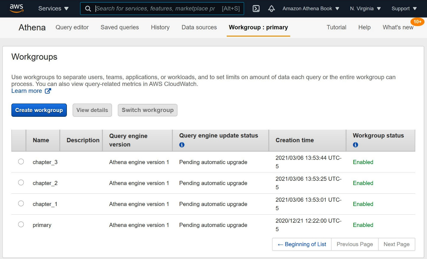
Figure 3.1 – The Athena WorkGroups screen
Athena customers often choose to use different WorkGroups for different kinds of queries. You can start getting into the habit of doing this right now by creating a new workgroup that you can use to run the remainder of the exercises in this book. To begin, click the Create workgroup button on the Workgroups page shown in Figure 3.1. You can get to that page by clicking on the Workgroup: primary tab at the top of the Athena console. If you are using the IAM policy recommended for this chapter, clicking the Create workgroup button will take you to a new page with the Create workgroup form, as shown in the following screenshot, Figure 3.2, and Figure 3.3:
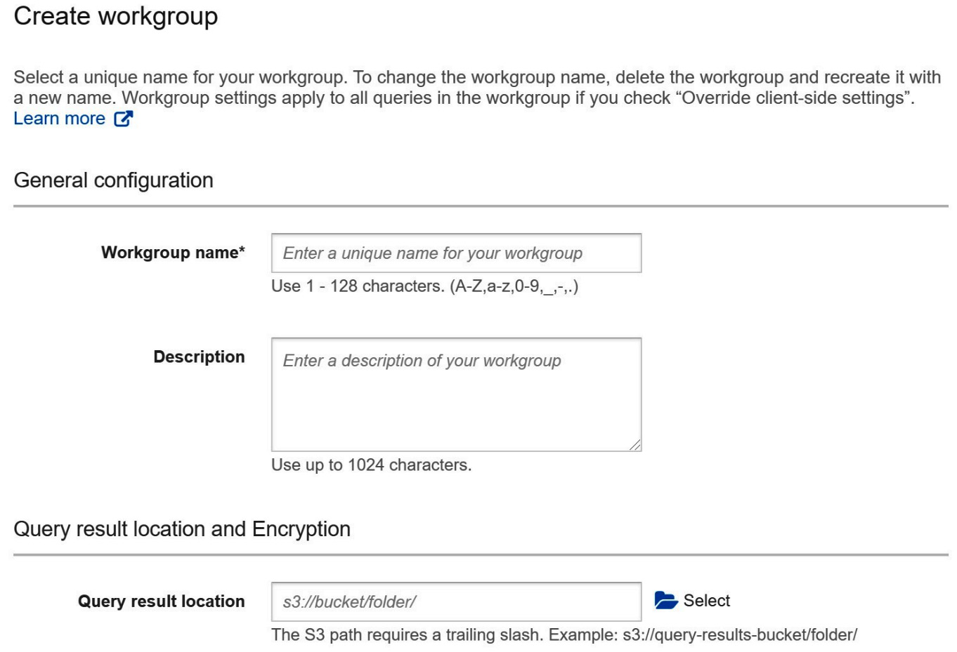
Figure 3.2 – Creating an Athena workgroup form Part 1
In Figure 3.2, you see the first three fields needed for workgroup creation. The first is simply the name of the new workgroup. The IAM policy recommended for this chapter will allow you to create new WorkGroups as long as they begin with packt-. You can try packt-athena-analytics as an example. The Description field is optional, purely used to document the purpose of the workgroup. Lastly, we need to set the default query results location for this workgroup. You may recall from previous chapters that Athena stores query results in S3 before making them available to your client or the Athena console. This allows you to reread the results as many times as you like, without needing to pay or wait for the query itself to run again. Naturally, we need to tell Athena where we'd like to store the results of queries run in this workgroup.
Aside from any organization naming conventions you may need to follow, there are two important factors to keep in mind when configuring these settings. The first is that Athena won't clean up this data after it's no longer needed. In fact, Athena has no idea if you are done using this data. You'll minimally want to set up an S3 Lifecycle policy to automatically delete data from this location that is older than a threshold you deem appropriate. If you need the results to be available longer than that, you should explicitly move them to a different location for long-term retention or consider running such queries in their own workgroup. Lastly, you'll want to consider who else has access to this S3 location. Imagine you have two personas in your organization: an Administrator who can read from any table and an intern who only has access to non-sensitive datasets. If the Administrator is running queries in a workgroup with a result location that is readable to the intern, you may be inadvertently providing a path for privilege escalation. The intern may accidentally stumble across the results of highly sensitive queries run by an Administrator. The same is true for a malicious actor. They no longer need to attack your permissioning system. You've unintentionally poked a hole in the armor by picking an overly permissive or shared query results location.
In the following screenshot, we are presented with four more settings to create our new workgroup:
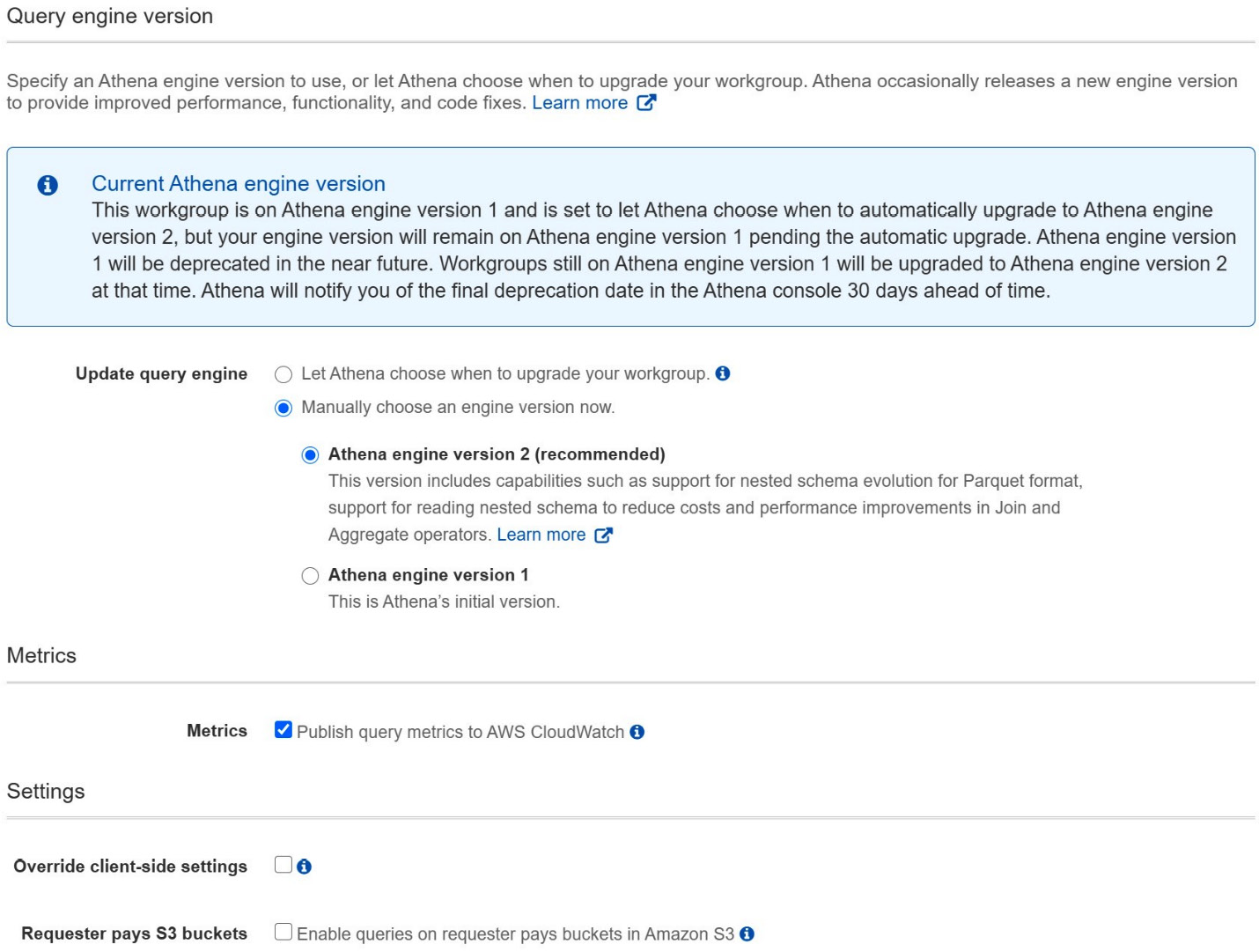
Figure 3.3 – Creating an Athena workgroup form Part 2
Athena's underlying engine, a hybrid of Presto and Trino, is rapidly evolving. As such, Athena has built-in facilities to handle upgrades. We'll talk more about Athena's automatic testing and upgrade functionality later in this chapter. For now, all you need to know is that Athena offers you full control over which engine version you use per workgroup. This allows you to isolate sensitive workloads to prevent auto-upgrades and enables you to take a sneak peek at upcoming versions so that you can prioritize upgrades that have an outsized benefit for you. It is highly recommended to set this to Let Athena choose when to upgrade your workgroup unless you've been advised otherwise by the Athena service team or are attempting to run a test against a specific version. This book's exercises will include new features that are only available in Athena engine version 2 or later, so be sure to pick Manually choose an engine version now and pick Athena engine version 2 or later. Failing to set the appropriate engine version on your workgroup may result in failures later, as Athena may or may not have auto-upgraded you when running through the exercises in this book.
The next setting determines if Athena will emit query metrics to AWS CloudWatch for all activities in the workgroup. We recommend leaving Metrics enabled as this will make troubleshooting, reporting, and auditing much easier. The last two settings are uncommon but enable interesting applications and integrations. As the Administrator of a workgroup, you can decide if clients can override workgroup-level settings such as results location on a per-query basis. The final setting controls whether Athena will allow queries in this workgroup to incur S3 charges that are typically paid by the owner of the S3 data itself. For example, if your company uses a separate AWS account per team and you query data that sits in another team's S3 bucket, that other team would typically be charged for any S3 operations or transfers that your query generates. Perhaps that other team doesn't like this billing model because it inflates their costs. After all, they didn't really run the query that incurred the usage cost. The data-providing team can set the bucket to Requester pays S3 buckets, which moves some of the charges to the account that accesses the S3 objects. You, as the customer, may not have signed off on these extra charges. This workgroup setting gives you control over what to do in these cases. By default, Athena will abort queries against S3 data configured to charge the requester. Toggling this setting changes that behavior.
The final option we can set on a workgroup is to apply resource tags. Tags allow you to organize resources across AWS services. Common uses involve billing, reporting, or simply understanding which projects make use of which resources. We won't be covering tagging in any depth here. Hence, we recommend leaving these blank as the recommended IAM policy for this chapter does not include creating or modifying tags. Once you are ready, you can click Create workgroup, as illustrated in the following screenshot, and your new workgroup should be ready to use. Don't forget to select that new workgroup by clicking Switch workgroup from Athena's workgroup page:
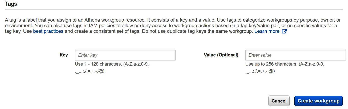
Figure 3.4 – Creating an Athena workgroup form Part 3
Now that we have our new packt-athena-analytics workgroup, let's see how we can save our most frequently used queries as named queries in our workgroup. Named Queries, also called saved queries in some parts of the Athena console, allow you to quickly load and run a query without re-entering the entire text of the query. To begin creating a named query, start typing a new query into the Athena query editor, just as you did for the previous queries we've run. For simplicity, you can use a COUNT(*) query by year over our taxi ride data, as illustrated in the following code snippet:
SELECT year, COUNT(*)
FROM packt_serverless_analytics.chapter_3_nyc_taxi_parquet
GROUP BY year
Go ahead and run the query so that we know it works and we didn't mistype anything. Once the query completes, click Save as below the query editor, as shown in the following screenshot:
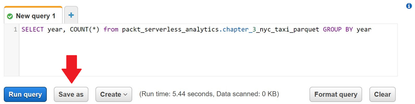
Figure 3.5 – Creating a named query
After you click Save as, you'll be prompted to give the query a name and a description. The saved query will only be visible to users of the workgroup you saved it to. Athena will remember this query and allow you to run or edit the query as many times as you like until you delete it. You can access the current set of saved queries by click on the saved queries tab at the top of the Athena console. This feature is good for bookmarking frequently used queries as part of an operational runbook or ad hoc analysis.
So far, all our Athena usage has been via the AWS console. As we begin to conclude Part 1 of this book, Fundamentals Of Amazon Athena, we'll introduce you to Athena's rich APIs. Virtually everything we've done with Athena's console can be done via the AWS software development kit (SDK) or AWS CLI. If you plan to build applications or automate analytics pipelines using Athena, you'll find using these APIs an easier route. If you aren't a developer or rarely use the command line, don't be intimidated. We will go step by step through each command, its arguments, and common reasons for failure.
Using Athena's APIs
As an introduction to Athena's APIs, we will demonstrate how to run basic geospatial queries with Athena using the AWS CLI. The AWS CLI provides a simple wrapper over each of the APIs supported by Athena. This allows us to get familiar with the APIs without having to make any choices about programming language. The APIs we use in this section are available in all supported languages such as Java, Golang, and Rust. Now that we've got a better understanding of the basic Athena concepts, we'll also use a slightly more advanced example dataset that will give us a chance to experiment with Athena's geospatial capabilities.
Use Athena engine version 2 or later
In case you skipped the instructions in the previous section pertaining to the creation of a new workgroup with Athena engine version 2, please take a moment to either switch to that workgroup now or change your current workgroup to explicitly use Athena engine version 2 or later to avoid errors in this exercise. Athena's geospatial functions have dramatically improved since Athena engine version1, so we'll be targeting features from Athena engine version 2 or later.
First, we will need to download two geospatial datasets from the Environmental Systems Research Institute (Esri), an industry leader in geospatial solutions, and upload that data to S3. The first dataset contains earthquake data for the state of California. The second dataset includes information on borders between all the different counties in California. California is an extremely seismically active area of the United States (US). Next, we will use Athena's APIs to run two Data Definition Language (DDL) queries to create tables for each of the datasets we downloaded. These datasets are less than 5 MB each. The book's GitHub repository contains a script that fully automates these steps to make this process easier. You can run the following commands in your AWS CloudShell environment, right from your browser. Alternatively, you can run these commands in most Linux-compatible environments with wget and the AWS CLI installed. After you run these commands, we'll quickly walk through what the geospatial_api_example.sh script does. Remember to supply the script with the S3 bucket you've been using to store data related to our experiments and the name of an Athena workgroup in which the script's queries will run:
wget -O geospatial_api_example.sh https://bit.ly/3sZZRia
chmod +x geospatial_api_example.sh
./geospatial_api_example.sh <S3_BUCKET> <ATHENA_WORKGROUP_NAME>
If successful, the script will have created two new tables in the packt_serverless_analytics database and printed the details of the accompanying Athena DDL queries to the Terminal. Let's go section by section through the script you downloaded earlier. We'll skip the uninteresting bits such as documentation or boilerplate error handling. Here we go:
#!/bin/bash
BUCKET=$1
WORKGROUP=$2
Bash scripts always start with a special sequence of characters, #!, called a shebang. This tells the system that what follows is a series of commands for a particular shell. In this case, we are using the Bash shell located at /bin/bash. This is mostly unrelated to Athena and its APIs, so don't worry if it is new or confusing. The only interesting bit in this first section is that the script treats the first argument as an S3 bucket and the second argument as an Athena workgroup. We'll see how these arguments get used later in the Athena APIs that get called.
The script then downloads the first dataset from the Esri GitHub repository using wget and then uploads it to S3 using the S3 bucket provided by the first argument to the script, as illustrated in the following code snippet. This process is repeated for the second dataset:
wget https://github.com/Esri/gis-tools-for-hadoop/blob/master/samples/data/earthquake-data/earthquakes.csv
aws s3 cp ./earthquakes.csv s3://$BUCKET/chapter_3/tables/earthquakes/
So far, the script hasn't interacted with Athena at all. This section prepares a CREATE TABLE query that it will send to Athena via the start-query-execution API. The script again uses some Bash magic in the form of read -d" VARIABLE << END_TOKEN to make the multiline CREATE TABLE query more human-readable. The code is illustrated here:
read -d '' create_earthquakes_table << EndOfMessage
CREATE external TABLE IF NOT EXISTS packt_serverless_analytics.chapter_3_earthquakes
(/* columns omitted for brevity */)
ROW FORMAT DELIMITED FIELDS TERMINATED BY ','
STORED AS TEXTFILE LOCATION 's3://${BUCKET}/chapter_3/tables/earthquakes/'
EndOfMessage
The CREATE TABLE query preparation is repeated for the second dataset before we finally get to our first Athena API calls. Here, we are using the start-query-execution API to run a DDL statement to create an earthquakes table. A nearly identical API call also gets made for the California counties dataset. The API takes two parameters, the query to run and the workgroup in which to run the query, as illustrated in the following code snippet:
aws athena start-query-execution
--query-string "${create_earthquakes_table}"
--work-group "${WORKGROUP}"
The vast majority of Athena's APIs are asynchronous. This means that the API calls complete relatively quickly, but the API's work isn't necessarily done when the API call completes. The start-query-execution API is a perfect example of this asynchronous pattern. When you run the script or this API call directly, you'll see that it returns almost immediately, even for queries that may take many minutes or hours to run. That's because completion of this API means Athena has accepted the query by doing some basic validations, authorization, and limit enforcement before giving us an identifier (ID) that we can later use to check the status of the query. This ID is called an Athena query execution ID and will also be used to retrieve our query's results programmatically.
Let's use the output of the script's two start-query-execution calls to check the status of our CREATE TABLE queries. Replace QueryExecutionId in the following command with one of your QueryExecutionId instances:
aws athena get-query-execution --query-execution-id <QueryExecutionId>
When you run this API call, you'll get output similar to the following. If your query ran into any issues, including permissions-related problems, you'd see root cause details too:
"QueryExecution": {
"Query": "<QUERY TEXT OMMITED FOR BREVITY>",
"StatementType": "DDL",
"ResultConfiguration": { "OutputLocation": "s3://… "},
"Status": {
"State": "SUCCEEDED",
"SubmissionDateTime": "2021-03-07T18:25:14.736000+00:00",
"CompletionDateTime": "2021-03-07T18:25:15.902000+00:00"
},
"Statistics": {
"DataScannedInBytes": 0,
"TotalExecutionTimeInMillis": 1166
},
"workgroup": "packt-athena-analytics"
}
In addition to giving us information about if the query succeeded or failed, the get-query-execution API also returns information about the type of query, how much data it scanned, how long it ran, and where its results were written. Using this API, you can embed lifecycle tracking and query scheduling functionality in your own applications. Now that we have a basic understanding of how to use Athena's APIs via the AWS CLI, let's try running queries that leverage Athena's geospatial functions. For this final exercise, let's imagine we work for an insurance company trying to build an automated claim-handling website. Our customers will go to this website and fill out forms to make insurance claims against their homeowners' insurance. We'd like to automatically approve or reject obvious claims before they get to a human. This saves time by giving customers rapid responses and helps ensure we prioritize essential claims. We've been asked to ensure that claims pertaining to natural disasters get escalated quickly. All our customers are in California, so we decided to start by automating earthquake claims. Whenever a customer selects earthquake as the cause for a claim, we need to run a query to determine if there were any recent earthquakes in their area. Luckily, Athena's geospatial function suite offers several ways to do this. A straightforward way is to understand if the county that the homeowner lives in has had any recent earthquakes. Here, we are using the county as a bounding box and then searching for any earthquakes in that vicinity. The ST_CONTAINS and ST_POINT functions allow us to treat the county as the search area and the earthquake's epicenter as a point; then, we can count how many earthquakes originated in each given county. In practice, a better method would also be to treat the earthquake as an area of impact and then the homeowner's house as a point, but that would be a much more challenging sample dataset to create.
The following Athena API call will run a query that uses our new earthquake and counties tables in conjunction with the ST_CONTAINS and ST_POINT functions to count how many earthquakes happened in each county:
aws athena start-query-execution
--query-string "SELECT counties.name, COUNT(*) cnt
FROM packt_serverless_analytics.chapter_3_counties as counties
CROSS JOIN packt_serverless_analytics.chapter_3_earthquakes as earthquakes
WHERE ST_CONTAINS (counties.boundaryshape, ST_POINT(earthquakes.longitude, earthquakes.latitude))
GROUP BY counties.name
ORDER BY cnt DESC"
--work-group "packt-athena-analytics"
If you repeat our get-query-execution API call for this query, you may see that it is in a RUNNING state since it takes much longer than our CREATE TABLE queries. You can keep running the get-query-execution API call shown here until the query transitions to a SUCCEEDED or FAILED state:
aws athena get-query-execution --query-execution-id <QueryExecutionId>
Assuming your query succeeds, you can then use Athena's get-query-results API to fetch pages of rows containing your query results. The command is shown in the following code block. Remember to substitute in a quoted version of your query's execution ID:
aws athena get-query-results --query-execution-id <QueryExecutionId>
The get-query-results API returns data as rows of JavaScript Object Notation (JSON) maps. The first row contains the column headers, while subsequent rows have the values associated with each row. The output can be very verbose, so many applications choose to access results directly from the S3 location. The code is illustrated in the following snippet:
{"ResultSet": { "Rows": [
{"Data": [{"VarCharValue": "name"},{"VarCharValue": "cnt"}]},
{"Data": [{"VarCharValue": "Kern"},{"VarCharValue": "36"}]},
{"Data": [{"VarCharValue": "San Bernardino"},{"VarCharValue":"35"}]}
...Remainder Omitted for Brevity...
When integrating with Athena, start-query-execution, get-query-execution, and get-query-results are the most frequently called APIs. Still, there are many others for managing WorkGroups and saving queries and data sources. Hopefully, if you've never used APIs before, this exercise has removed some of the mystery surrounding them. If you're a seasoned developer, you're likely starting to form a view of how you can connect your applications to Athena. Chapter 9, Serverless ETL Pipelines, and Chapter 10, Building Applications with Amazon Athena, will use more sophisticated examples to demonstrate the power of integrating your application with Athena.
Summary
In this chapter, you concluded your introduction to Athena by getting hands-on with the key features that will allow you to use Athena for many everyday analytics tasks. We practiced queries and techniques that add new data, either in bulk via CTAS or incrementally through INSERT INTO, to our data lake. Our exercises also included experiments with approximate query techniques that improve our ability to find insights in our data. Features such as TABLESAMPLE or approx_percentile allow us to trade query accuracy for reduced cost or shorter runtimes. Cheaper and faster exploration queries enable us to consult the data more often. This leads to better decision-making and less reluctance to run long or expensive queries because you proved their worth with a shorter, approximate query. This may be hard to imagine given that all the queries in this chapter took less than a minute to run and, in aggregate, cost less than USD 1. In practice, many fascinating queries can take hours or days to complete and cost hundreds of dollars. These are the cases where approximate query techniques can show their merit.
Next, we saw how to organize our workloads into WorkGroups so that our queries can use different settings such as Athena engine. Then, we closed out with an excursion into using Athena's APIs, instead of the AWS console, to run queries. This example was simple but demonstrated how a fictional insurance company could use these APIs to enhance their application by running geospatial workloads on Athena.
While your introduction to Athena is now complete, the next part of this book will begin an introduction to building data lakes at scale. Understanding how data modeling affects your Athena applications' performance and security will enable you to ensure you have the right data in place for your application or analytics needs. Tools such as AWS Lake Formation will help you automate many of the activities you'll need to have in place before Part 3 of this book, Using Amazon Athena, brings us full circle to write our applications on top of Athena.