So far, we've learned how to build deep neural networks and the impact of tweaking their various hyperparameters. In this chapter, we will learn about where traditional deep neural networks do not work. We'll then learn about the inner workings of convolutional neural networks (CNNs) by using a toy example before understanding some of their major hyperparameters, including strides, pooling, and filters. Next, we will leverage CNNs, along with various data augmentation techniques, to solve the issue of traditional deep neural networks not having good accuracy. Following this, we will learn about what the outcome of a feature learning process in a CNN looks like. Finally, we'll put our learning together to solve a use case: we'll be classifying an image by stating whether the image contains a dog or a cat. By doing this, we'll be able to understand how the accuracy of prediction varies by the amount of data available for training.
The following topics will be covered in this chapter:
- The problem with traditional deep neural networks
- Building blocks of a CNN
- Implementing a CNN
- Classifying images using deep CNNs
- Implementing data augmentation
- Visualizing the outcome of feature learning
- Building a CNN for classifying real-world images
Let's get started!
The problem with traditional deep neural networks
Before we dive into CNNs, let's look at the major problem that's faced when using traditional deep neural networks.
Let's reconsider the model we built on the Fashion-MNIST dataset in Chapter 3, Building a Deep Neural Network with PyTorch. We will fetch a random image and predict the class that corresponds to that image, as follows:
- Fetch a random image from the available training images:
# Note that you should run the code in
# Batch size of 32 section in Chapter 3
# before running the following code
import matplotlib.pyplot as plt
%matplotlib inline
# ix = np.random.randint(len(tr_images))
ix = 24300
plt.imshow(tr_images[ix], cmap='gray')
plt.title(fmnist.classes[tr_targets[ix]])
The preceding code results in the following output:

- Pass the image through the trained model (continue using the model we trained in the Batch size of 32 section of Chapter 3, Building a Deep Neural Network with PyTorch).
- Preprocess the image so it goes through the same pre-processing steps we performed while building the model:
img = tr_images[ix]/255.
img = img.view(28*28)
img = img.to(device)
- Extract the probabilities associated with the various classes:
np_output = model(img).cpu().detach().numpy()
np.exp(np_output)/np.sum(np.exp(np_output))
The preceding code results in the following output:

From the preceding output, we can see that the highest probability is for the 1st index, which is of the Trouser class.
- Translate (roll/slide) the image multiple times (one pixel at a time) from a translation of 5 pixels to the left to 5 pixels to the right and store the predictions in a list.
- Create a list that stores predictions:
preds = []
- Create a loop that translates (rolls) an image from -5 pixels (5 pixels to the left) to +5 pixels (5 pixels to the right) of the original position (which is at the center of the image):
for px in range(-5,6):
In the preceding code, we specified 6 as the upper bound, even though we are interested in translating until +5 pixels, since the output of the range would be from -5 to +5 when (-5,6) is the specified range.
- Pre-process the image, as we did in step 2:
    img = tr_images[ix]/255.
    img = img.view(28, 28)
- Roll the image by a value equal to px within the for loop:
img2 = np.roll(img, px, axis=1)
In the preceding code, we specified axis=1 since we want the image pixels to be moving horizontally and not vertically.
- Store the rolled image as a tensor object and register it to device:
img3 = torch.Tensor(img2).view(28*28).to(device)
- Pass img3 through the trained model to predict the class of the translated (rolled) image and append it to the list that is storing predictions for various translations:
    np_output = model(img3).cpu().detach().numpy()
    preds.append(np.exp(np_output)/np.sum(np.exp(np_output)))
- Visualize the predictions of the model for all the translations (-5 pixels to +5 pixels):
import seaborn as sns
fig, ax = plt.subplots(1,1, figsize=(12,10))
plt.title('Probability of each class
for various translations')
sns.heatmap(np.array(preds), annot=True, ax=ax, fmt='.2f',
            xticklabels=fmnist.classes,
            yticklabels=[str(i)+str(' pixels')
                         for i in range(-5,6)], cmap='gray')
The preceding code results in the following output:

Now that we have learned about a scenario where a traditional neural network fails, we will learn about how CNNs help address this problem. But before we do this, we will learn about the building blocks of a CNN.
Building blocks of a CNN
CNNs are the most prominent architectures that are used when working on images. CNNs address the major limitations of deep neural networks that we saw in the previous section. Besides image classification, they also help with object detection, image segmentation, GANs, and many more – essentially, wherever we use images. Furthermore, there are different ways of constructing a convolutional neural network, and there are multiple pre-trained models that leverage CNNs to perform various tasks. Starting with this chapter, we will be using CNNs extensively.
In the upcoming subsections, we will understand the fundamental building blocks of a CNN, which are as follows:
- Convolutions
- Filters
- Strides and padding
- Pooling
Let's get started!
Convolution
A convolution is basically multiplication between two matrices. As you saw in the previous chapter, matrix multiplication is a key ingredient of training a neural network. (We perform matrix multiplication when we calculate hidden layer values – which is a matrix multiplication of the input values and weight values connecting the input to the hidden layer. Similarly, we perform matrix multiplication to calculate output layer values.)
To ensure we have a solid understanding of the convolution process, let's go through the following example.
Let's assume we have two matrices we can use to perform convolution.
Here is Matrix A:

Here is Matrix B:

While performing the convolution operation, you are sliding Matrix B (the smaller matrix) over Matrix A (the bigger matrix). Furthermore, we are performing element to element multiplication between Matrix A and Matrix B, as follows:
- Multiply {1,2,5,6} of the bigger matrix by {1,2,3,4} of the smaller matrix:
1*1 + 2*2 + 5*3 + 6*4 = 44
- Multiply {2,3,6,7} of the bigger matrix by {1,2,3,4} of the smaller matrix:
2*1 + 3*2 + 6*3 + 7*4 = 54
- Multiply {3,4,7,8} of the bigger matrix by {1,2,3,4} of the smaller matrix:
3*1 + 4*2 + 7*3 + 8*4 = 64
- Multiply {5,6,9,10} of the bigger matrix by {1,2,3,4} of the smaller matrix:
5*1 + 6*2 + 9*3 + 10*4 = 84
- Multiply {6,7,10,11} of the bigger matrix by {1,2,3,4} of the smaller matrix:
- Multiply {7,8,11,12} of the bigger matrix by {1,2,3,4} of the smaller matrix:
- Multiply {9,10,13,14} of the bigger matrix by {1,2,3,4} of the smaller matrix:
- Multiply {10,11,14,15} of the bigger matrix by {1,2,3,4} of the smaller matrix:
- Multiply {11,12,15,16} of the bigger matrix by {1,2,3,4} of the smaller matrix:
11*1 + 12*2 + 15*3 + 16*4 = 144
The result of performing the preceding operations is as follows:

The smaller matrix is typically called a filter or a kernel, while the bigger matrix is the original image.
Filter
A filter is a matrix of weights that is initialized randomly at the start. The model learns the optimal weight values of a filter over increasing epochs.
The concept of filters brings us to two different aspects:
- What the filters learn about
- How filters are represented
In general, the more filters there are in a CNN, the more features of an image that the model can learn about. We will learn about what various filters learn in the Visualizing the filters' learning section of this chapter. For now, we'll ensure that we have an intermediate understanding that the filters learn about different features present in the image. For example, a certain filter might learn about the ears of a cat and provide high activation (a matrix multiplication value) when the part of the image it is convolving with contains the ear of a cat.
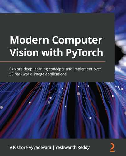
In the previous section, we learned that when we convolved one filter that has a size of 2 x 2 with a matrix that has a size of 4 x 4, we got an output that is 3 x 3 in dimension.
However, if 10 different filters multiply the bigger matrix (original image), the result is 10 sets of the 3 x 3 output matrices.
Furthermore, in a scenario where we are dealing with color images where there are three channels, the filter that is convolving with the original image would also have three channels, resulting in a single scalar output per convolution. Also, if the filters are convolving with an intermediate output – let's say of 64 x 112 x 112 in shape – the filter would have 64 channels to fetch a scalar output. In addition, if there are 512 filters that are convolving with the output that was obtained in the intermediate layer, the output post convolution with 512 filters would be 512 x 111 x 111 in shape.
To solidify our understanding of the output of filters further, let's take a look at the following diagram:
In the preceding diagram, we can see that the input image is multiplied by the filters that have the same depth as that of the input (which the filters are convolving with) and that the number of channels in the output of a convolution is as many as there are filters.
Strides and padding
In the previous section, each filter strode across the image – one column and one row at a time (after exhausting all possible columns by the end of the image). This also resulted in the output size being 1 pixel less than the input image size – both in terms of height and width. This results in a partial loss of information and can affect the possibility of us adding the output of the convolution operation to the original image (this is known as residual addition and will be discussed in detail in the next chapter).
In this section, we will learn about how strides and padding influence the output shape of convolutions.
Strides
Let's understand the impact of stride by leveraging the same example that we saw in the Filter section. Furthermore, we'll stride Matrix B with a stride of 2 over Matrix A. The output of convolution with a stride of 2 is as follows:
- {1,2,5,6} of the bigger matrix is multiplied by {1,2,3,4} of the smaller matrix:
1*1 + 2*2 + 5*3 + 6*4 = 44
- {3,4,7,8} of the bigger matrix is multiplied by {1,2,3,4} of the smaller matrix:
3*1 + 4*2 + 7*3 + 8*4 = 64
- {9,10,13,14} of the bigger matrix is multiplied by {1,2,3,4} of the smaller matrix:
- {11,12,15,16} of the bigger matrix is multiplied by {1,2,3,4} of the smaller matrix:
11*1 + 12*2 + 15*3 + 16*4 = 144
The result of performing the preceding operations is as follows:

Note that the preceding output has a lower dimension compared to the scenario where the stride was 1 (where the output shape was 3 x 3) since we now have a stride of 2.
Padding
In the preceding case, we could not multiply the leftmost elements of the filter by the rightmost elements of the image. If we were to perform such matrix multiplication, we would pad the image with zeros. This would ensure that we can perform element to element multiplication of all the elements within an image with a filter.
Let's understand padding by using the same example we used in the Convolution section.
Once we add padding on top of Matrix A, the revised version of Matrix A will look as follows:

From the preceding matrix, we can see that we have padded Matrix A with zeros and that the convolution with Matrix B will not result in the output dimension being smaller than the input's dimension. This aspect comes in handy when we are working on residual network where we must add the output of the convolution to the original image.
Once we've done this, we can perform activation on top of the convolution operation's output. We could use any of the activation functions we saw in Chapter 3, Building a Deep Neural Network with PyTorch, for this.
Pooling
Pooling aggregates information in a small patch. Imagine a scenario where the output of convolution activation is as follows:

The max pooling for this patch is 4. Here, we have considered the elements in this pool of elements and have taken the maximum value across all the elements present.
Similarly, let's understand the max pooling for a bigger matrix:

In the preceding case, if the pooling stride has a length of 2, the max pooling operation is calculated as follows, where we divide the input image by a stride of 2 (that is, we have divided the image into 2 x 2 divisions):

For the four sub-portions of the matrix, the maximum values in the pool of elements are as follows:

In practice, it is not necessary to always have a stride of 2; this has just been used for illustration purposes here.
Other variants of pooling are sum and average pooling. However, in practice, max pooling is used more often.
Note that by the end of performing the convolution and pooling operations, the size of the original matrix is reduced from 4 x 4 to 2 x 2. In a realistic scenario, if the original image is of shape 200 x 200 and the filter is of shape 3 x 3, the output of the convolution operation would be 198 x 198. After that, the output of the pooling operation with a stride of 2 is 99 X 99.
Putting them all together
So far, we have learned about convolution, filters, and pooling, and their impact in reducing the dimension of an image. Now, we will learn about another critical component of a CNN – the flatten layer (fully connected layer) – before putting the three pieces we have learned about together.
To understand the flattening process, we'll take the output of the pooling layer in the previous section and flatten the output. The output of flattening the pooling layer is as follows:
{6, 8, 14, 16}
By doing this, we'll see that the flatten layer can be treated equivalent to the input layer (where we flattened the input image into a 784-dimensional input in Chapter 3, Building a Deep Neural Network with PyTorch). Once the flatten layer's (fully connected layer) values have been obtained, we can pass it through the hidden layer and then obtain the output for predicting the class of an image.
The overall flow of a CNN is as follows:

In the preceding image, we can see the overall flow of a CNN model, where we are passing an image through convolution via multiple filters and then pooling (and in the preceding case, repeating the convolution and pooling process twice), before flattening the output of the final pooling layer. This forms the feature learning part of the preceding image.
The operations of convolution and pooling constitute the feature learning section as filters help in extracting relevant features from images and pooling helps in aggregating information and thereby reducing the number of nodes at the flatten layer. (If we directly flatten the input image (which is 300 x 300 pixels in size, for example), we are dealing with 90K input values. If we have 90K input pixel values and 100K nodes in a hidden layer, we are looking at ~9 billion parameters, which is huge in terms of computation.)
Convolution and pooling help in fetching a flattened layer that has a much smaller representation than the original image.
Finally, the last part of the classification is similar to the way we classified images in Chapter 3, Building a Deep Neural Network in PyTorch, where we had a hidden layer and then obtained the output layer.
How convolution and pooling help in image translation
When we perform pooling, we can consider the output of the operation as an abstraction of a region (a small patch). This phenomenon comes in handy, especially when images are being translated.
Think of a scenario where an image is translated by 1 pixel to the left. Once we perform convolution, activation, and pooling on top of it, we'll have reduced the dimension of the image (due to pooling), which means that a fewer number of pixels store the majority of the information from the original image. Moreover, given that pooling stores information of a region (patch), the information within a pixel of the pooled image would not vary, even if the original image is translated by 1 unit. This is because the maximum value of that region is likely to get captured in the pooled image.
Convolution and pooling cam also help us with the receptive field. To understand the receptive field, let's imagine a scenario where we perform a convolution pooling operation twice on an image that is 100 x 100 in shape. The output at the end of the two convolution pooling operations is of the shape 25 x 25 (if the convolution operation was done with padding). Each cell in the 25 x 25 output now corresponds to a larger 4 x 4 portion of the original image. Thus, because of the convolution and pooling operations, each cell in the resulting image corresponds to a patch of the original image.
Now that we have learned about the core components of a CNN, let's apply them all to a toy example to understand how they work together.
Implementing a CNN
A CNN is one of the foundational blocks of computer vision techniques, and it is important for you to have a solid understanding of how they work. While we already know that a CNN constitutes convolution, pooling, flattening, and then the final classification layer, in this section, we will understand the various operations that occur during the forward pass of a CNN through code.
To gain a solid understanding of this, first, we will build a CNN architecture on a toy example using PyTorch and then match the output by building the feed-forward propagation from scratch in Python.
Building a CNN-based architecture using PyTorch
The CNN architecture will differ from the neural network architecture that we built in the previous chapter in that a CNN constitutes the following in addition to what a typical vanilla deep neural network would have:
- Convolution operation
- Pooling operation
- Flattening layer
In the following code, we will build a CNN model on a toy dataset, as follows:
- First, we need to import the relevant libraries:
import torch
from torch import nn
from torch.utils.data import TensorDataset, Dataset, DataLoader
from torch.optim import SGD, Adam
device = 'cuda' if torch.cuda.is_available() else 'cpu'
from torchvision import datasets
import numpy as np
import matplotlib.pyplot as plt
%matplotlib inline
- Then, we need to create the dataset using the following steps:
X_train = torch.tensor([[[[1,2,3,4],[2,3,4,5],
                          [5,6,7,8],[1,3,4,5]]],
                [[[-1,2,3,-4],[2,-3,4,5],
            [-5,6,-7,8],[-1,-3,-4,-5]]]]).to(device).float()
X_train /= 8
y_train = torch.tensor([0,1]).to(device).float()
Here, we are scaling the input dataset so that it has a range between -1 to +1 by dividing the input data by the maximum input value; that is, 8.
The shape of the input dataset is (2,1,4,4) since there are two data points, where each is 4 x 4 in shape and has 1 channel.
- Define the model architecture:
def get_model():
    model = nn.Sequential(
                nn.Conv2d(1, 1, kernel_size=3),
                nn.MaxPool2d(2),
                nn.ReLU(),
                nn.Flatten(),
                nn.Linear(1, 1),
                nn.Sigmoid(),
            ).to(device)
    loss_fn = nn.BCELoss()
    optimizer = Adam(model.parameters(), lr=1e-3)
    return model, loss_fn, optimizer
Note that in the preceding model, we are specifying that there is 1 channel in the input and that we are extracting 1 channel from the output post convolution (that is, we have 1 filter with a size of 3 x 3) using the nn.Conv2d method. After this, we perform max pooling using nn.MaxPool2d and ReLU activation (using nn.Relu()) prior to flattening and connecting to the final layer, which has one output per data point.
Furthermore, note that the loss function is binary cross-entropy loss (nn.BCELoss()) since the output is from a binary class. We are also specifying that the optimization will be done using the Adam optimizer with a learning rate of 0.001.
- Summarize the architecture of the model using the summary method that's available in the torch_summary package post fetching our model, loss function (loss_fn), and optimizer by calling the get_model function:
!pip install torch_summary
from torchsummary import summary
model, loss_fn, optimizer = get_model()
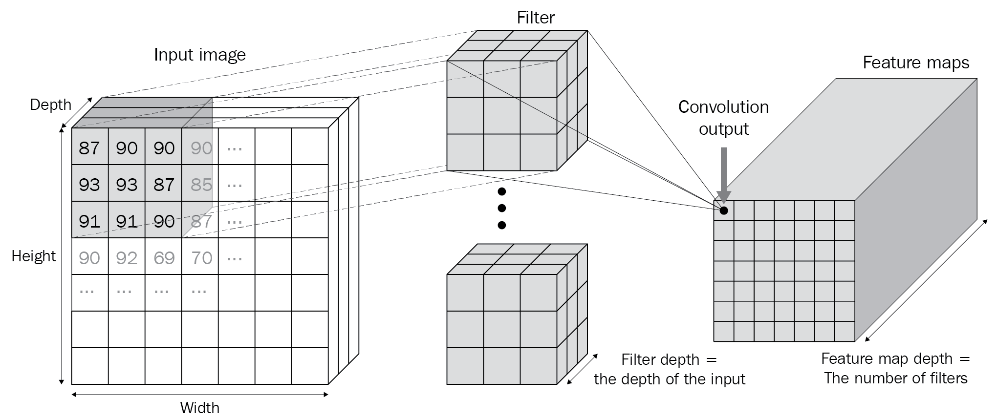
summary(model, X_train);
The preceding code results in the following output:
Let's understand the reason why each layer contains so many parameters. The arguments of the Conv2d class are as follows:

In the preceding case, we are specifying that the size of the convolving kernel (kernel_size) is 3 and that the number of out_channels is 1 (essentially, the number of filters is 1), where the number of initial (input) channels is 1. Thus, for each input image, we are convolving a filter of shape 3 x 3 on a shape of 1 x 4 x 4, which results in an output of the shape 1 x 2 x 2. There are 10 parameters since we are learning the nine weight parameters (3 x 3) and the one bias of the convolving kernel. For the MaxPool2d, ReLU, and Flatten layers, there are no parameters as these are operations that are performed on top of the output of the convolution layer; no weights or biases are involved.
- The linear layer has two parameters – one weight and one bias – which means there's a total of 12 parameters (10 from the convolution operation and two from the linear layer).
- Train the model using the same model training code we used in Chapter 3, Building a Deep Neural Network with PyTorch, where we defined the function that will train on batches of data (train_batch). Then, fetch the DataLoader and train it on batches of data over 2,000 epochs (we're only using 2,000 because this is a small toy dataset), as follows:
- Define the function that will train on batches of data (train_batch):
def train_batch(x, y, model, opt, loss_fn):
    model.train()
    prediction = model(x)
    batch_loss = loss_fn(prediction.squeeze(0), y)
    batch_loss.backward()
    optimizer.step()
    optimizer.zero_grad()
    return batch_loss.item()
- Define the training DataLoader by specifying the dataset using the TensorDataset method and then loading it using DataLoader:
trn_dl = DataLoader(TensorDataset(X_train, y_train))
Note that, given we are not modifying the input data by a lot, we won't be building a class separately, instead leveraging the TensorDataset method directly, which provides an object that corresponds to the input data.
- Train the model over 2,000 epochs:
for epoch in range(2000):
    for ix, batch in enumerate(iter(trn_dl)):
        x, y = batch
        batch_loss = train_batch(x, y, model, optimizer,
                                 loss_fn)
With the preceding code, we have trained the CNN model on our toy dataset.
- Perform a forward pass on top of the first data point:
model(X_train[:1])
The output of the preceding code is 0.1625.
In the next section, we will learn about how forward propagation in CNNs works so that we can obtain a value of 0.1625 on the first data point.
Forward propagating the output in Python
Before we proceed, note that this section is only here to help you clearly understand how CNNs work. We don't need to perform the following steps in a real-world scenario:
- Extract the weights and biases of the convolution and linear layers of the architecture that's been defined, as follows:
- Extract the various layers of the model:
list(model.children())
This results in the following output:

- Extract the layers among all the layers of the model that have the weight attribute associated with them:
(cnn_w, cnn_b), (lin_w, lin_b) = [(layer.weight.data,
                            layer.bias.data) for layer in
                            list(model.children())
                                  if hasattr(layer,'weight')]
In the preceding code, hasattr(layer,'weight') returns a boolean, regardless of whether the layer contains the weight attribute.
Note that the convolution (Conv2d) layer and the Linear layer at the end are the only layers that contain parameters, which is why we saved them as cnn_w and cnn_b for the Conv2d layer and lin_w and lin_b for the Linear layer, respectively.
The shape of cnn_w is 1 x 1 x 3 x 3 since we have initialized one filter, which has one channel and a dimension of 3 x 3. cnn_b has a shape of 1 as it corresponds to one filter.
- To perform the cnn_w convolution operation over the input value, we must initialize a matrix of zeros for sumproduct (sumprod) where the height is input height - filter height + 1 and the width is width - filter width + 1:
h_im, w_im = X_train.shape[2:]
h_conv, w_conv = cnn_w.shape[2:]
sumprod = torch.zeros((h_im - h_conv + 1, w_im - w_conv + 1))
- Now, let's fill sumprod by convoluting the filter (cnn_w) across the first input and summing up the filter bias term (cnn_b) after reshaping the filter shape from a 1 x 1 x 3 x 3 shape to a 3 x 3 shape:
for i in range(h_im - h_conv + 1):
    for j in range(w_im - w_conv + 1):
        img_subset = X_train[0, 0, i:(i+3), j:(j+3)]
        model_filter = cnn_w.reshape(3,3)
        val = torch.sum(img_subset*model_filter) + cnn_b
        sumprod[i,j] = val
In the preceding code, img_subset stores the portion of the input that we would be convolving with the filter and hence we stride through it across the possible columns and then rows.
Furthermore, given that the input is 4 x 4 in shape and the filter is 3 x 3 in shape, the output is 2 x 2 in shape.
At this stage, the output of sumprod is as follows:

- Perform the ReLU operation on top of the output and then fetch the maximum value of the pool (MaxPooling), as follows:
- ReLU is performed on top of sumprod in Python as follows:
sumprod.clamp_min_(0)
Note that we are clamping the output to a minimum of 0 in the preceding code (which is what ReLU activation does):

- The output of the pooling layer can be calculated like so:
pooling_layer_output = torch.max(sumprod)
The preceding code results in the following output:
- Pass the preceding output through linear activation:
intermediate_output_value = pooling_layer_output*lin_w+lin_bThe output of this operation is as follows:
- Pass the output through the sigmoid operation:
from torch.nn import functional as F # torch library
# for numpy like functions
print(F.sigmoid(intermediate_output_value))
The preceding code gives us the following output:
Note that we perform sigmoid and not softmax since the loss function is binary cross-entropy and not categorical cross-entropy like it was in the Fashion-MNIST dataset.
The preceding code gives us the same output we obtained using PyTorch's feedforward method, thus strengthening our understanding of how CNNs work.
Now that we have learned about how CNNs work, in the next section, we'll apply this to the Fashion-MNIST dataset and see how it fares on translated images.
Classifying images using deep CNNs
So far, we have seen that the traditional neural network predicts incorrectly for translated images. This needs to be addressed because in real-world scenarios, various augmentations will need to be applied, such as translatation and rotation, that were not seen during the training phase. In this section, we will understand how CNNs address the problem of incorrect predictions when image translation happens on images in the Fashion-MNIST dataset.
The pre-processing portion of the Fashion-MNIST dataset remains the same as in the previous chapter, except that when we reshape (.view) the input data, instead of flattening the input to 28 x 28 = 784 dimensions, we reshape the input to a shape of (1,28,28) for each image (remember, channels are to be specified first, followed by their height and width, in PyTorch):
- Import the necessary packages:
from torchvision import datasets
from torch.utils.data import Dataset, DataLoader
import torch
import torch.nn as nn
device = "cuda" if torch.cuda.is_available() else "cpu"
import numpy as np
import matplotlib.pyplot as plt
%matplotlib inline

data_folder = '~/data/FMNIST' # This can be any directory you
# want to download FMNIST to
fmnist = datasets.FashionMNIST(data_folder, download=True,
                                        train=True)
tr_images = fmnist.data
tr_targets = fmnist.targets
- The Fashion-MNIST dataset class is defined as follows. Remember, the Dataset object will always need the __init__, __getitem__, and __len__ methods we've defined:
class FMNISTDataset(Dataset):
    def __init__(self, x, y):
        x = x.float()/255
        x = x.view(-1,1,28,28)
        self.x, self.y = x, y
    def __getitem__(self, ix):
        x, y = self.x[ix], self.y[ix]
        return x.to(device), y.to(device)
    def __len__(self):
        return len(self.x)
The preceding line of code in bold is where we are reshaping each input image (differently to what we did in the previous chapter) since we are providing data to a CNN that expects each input to have a shape of batch size x channels x height x width.
- The CNN model architecture is defined as follows:
from torch.optim import SGD, Adam
def get_model():
    model = nn.Sequential(
                nn.Conv2d(1, 64, kernel_size=3),
                nn.MaxPool2d(2),
                nn.ReLU(),
                nn.Conv2d(64, 128, kernel_size=3),
                nn.MaxPool2d(2),
                nn.ReLU(),
                nn.Flatten(),
                nn.Linear(3200, 256),
                nn.ReLU(),
                nn.Linear(256, 10)
            ).to(device)

    loss_fn = nn.CrossEntropyLoss()
    optimizer = Adam(model.parameters(), lr=1e-3)
    return model, loss_fn, optimizer
- A summary of the model can be created using the following code:
!pip install torch_summary
from torchsummary import summary
model, loss_fn, optimizer = get_model()
summary(model, torch.zeros(1,1,28,28));
This results in the following output:

To solidify our understanding of CNNs, let's understand the reason why the number of parameters have been set the way they have in the preceding output:
- Layer 1: Given that there are 64 filters with a kernel size of 3, we have 64 x 3 x 3 weights and 64 x 1 biases, resulting in a total of 640 parameters.
- Layer 4: Given that there are 128 filters with a kernel size of 3, we have 128 x 64 x3 x 3 weights and 128 x 1 biases, resulting in a total of 73,856 parameters.
- Layer 8: Given that a layer with 3,200 nodes is getting connected to another layer with 256 nodes, we have a total of 3,200 x 256 weights + 256 biases, resulting in a total of 819,456 parameters.
- Layer 10: Given that a layer with 256 nodes is getting connected to a layer with 10 nodes, we have a total of 256 x 10 weights and 10 biases, resulting in a total of 2,570 parameters.
Once the model has been trained, you'll notice that the variation of accuracy and loss over the training and test datasets is as follows:

Note that in the preceding scenario, the accuracy of the validation dataset is ~92% within the first five epochs, which is already better than the accuracy we saw across various techniques in the previous chapter, even without additional regularization.
Now, let's translate the image and predict the class of translated images:
- Translate the image between -5 pixels to +5 pixels and predict its class:
preds = []
ix = 24300
for px in range(-5,6):
    img = tr_images[ix]/255.
    img = img.view(28, 28)
    img2 = np.roll(img, px, axis=1)
    plt.imshow(img2)
    plt.show()
    img3 = torch.Tensor(img2).view(-1,1,28,28).to(device)
    np_output = model(img3).cpu().detach().numpy()
    preds.append(np.exp(np_output)/np.sum(np.exp(np_output)))
In the preceding code, we reshaped the image (img3) so that it has a shape of (-1,1,28,28) so that we can pass the image to a CNN model.
- Plot the probability of the classes across various translations:
import seaborn as sns
fig, ax = plt.subplots(1,1, figsize=(12,10))
plt.title('Probability of each class for
various translations')
sns.heatmap(np.array(preds).reshape(11,10), annot=True,
            ax=ax, fmt='.2f', xticklabels=fmnist.classes,
            yticklabels=[str(i)+str(' pixels')
                         for i in range(-5,6)], cmap='gray')
The preceding code results in the following output:

Note that in this scenario, even when the image was translated by 4 pixels, the prediction was correct, while in the scenario where we did not use a CNN, the prediction was incorrect when the image was translated by 4 pixels. Furthermore, when the image was translated by 5 pixels, the probability of "Trouser" dropped considerably.
As we can see, while CNNs help in addressing the challenge of image translation, they don't solve the problem at hand completely. We will learn how to address such a scenario by leveraging data augmentation alongside CNNs in the next section.
Implementing data augmentation
In the previous scenario, we learned about how CNNs help in predicting the class of an image when it is translated. While this worked well for translations of up to 5 pixels, anything beyond that is likely to have a very low probability for the right class. In this section, we'll learn how to ensure that we predict the right class, even if the image is translated by a considerable amount.
To address this challenge, we'll train the neural network by translating the input images by 10 pixels randomly (both toward the left and the right) and passing them to the network. This way, the same image will be processed as a different image in different passes since it will have had a different amount of translation in each pass.
Before we leverage augmentations to improve the accuracy of our model when images are translated, let's learn about the various augmentations that can be done on top of an image.
Image augmentations
So far, we have learned about the issues image translation can have on a model's prediction accuracy. However, in the real world, we might encounter various scenarios, such as the following:
- Images are rotated slightly
- Images are zoomed in/out (scaled)
- Some amount of noise is present in the image
- Images have low brightness
- Images have been flipped
- Images have been sheared (one side of the image is more twisted)
A neural network that does not take the preceding scenarios into consideration won't provide accurate results, just like in the previous section, where we had a neural network that had not been explicitly trained on images that had been heavily translated.
The augmenters class in the imgaug package has useful utilities for performing these augmentations. Let's take a look at the various utilities present in the augmenters class for generating augmented images from a given image. Some of the most prominent augmentation techniques are as follows:
- Affine transformations
- Change brightness
- Add noise
Affine transformations
Affine transformations involve translating, rotating, scaling, and shearing an image. They can be performed in code using the Affine method that's present in the augmenters class. Let's take a look at the parameters present in the Affine method by looking at the following screenshot. Here, we have defined all the parameters of the Affine method:

Some of the important parameters in the Affine method are as follows:
- scale specifies the amount of zoom that is to be done for the image
- translate_percent specifies the amount of translation as a percentage of the image's height and width
- translate_px specifies the amount of translation as an absolute number of pixels
- rotate specifies the amount of rotation that is to be done on the image
- shear specifies the amount of rotation that is to be done on part of the image
Before we consider ay other parameters, let's understand where scaling, translation, and rotation come in handy.
Fetch a random image from the training dataset for fashionMNIST:
- Download images from the Fashion-MNIST dataset:
from torchvision import datasets
import torch
data_folder = '/content/' # This can be any directory
# you download FMNIST to
fmnist = datasets.FashionMNIST(data_folder, download=True,
                               train=True)
- Fetch an image from the downloaded dataset:
tr_images = fmnist.data
tr_targets = fmnist.targets
- Let's plot the first image:
import matplotlib.pyplot as plt
%matplotlib inline
plt.imshow(tr_images[0])
The output of the preceding code is as follows:

Perform scaling on top of the image:
- Define an object that performs scaling:
from imgaug import augmenters as iaa
aug = iaa.Affine(scale=2)
- Specify that we want to augment the image using the augment_image method, which is available in the aug object, and plot it:
plt.imshow(aug.augment_image(tr_images[0]))
plt.title('Scaled image')
The output of the preceding code is as follows:

In the preceding output, the image has been zoomed into considerably. This has resulted in some pixels being cut from the original image since the output shape of the image hasn't changed.
Now, let's take a look at a scenario where an image has been translated by a certain number of pixels using the translate_px parameter:
aug = iaa.Affine(translate_px=10)
plt.imshow(aug.augment_image(tr_images[0]))
plt.title('Translated image by 10 pixels')
The output of the preceding code is as follows:

In the preceding output, the translation by 10 pixels has happened across both the x and y axes.
If we want to perform translation more in one axis and less in the other axis, we must specify the amount of translation we want in each axis:
aug = iaa.Affine(translate_px={'x':10,'y':2})
plt.imshow(aug.augment_image(tr_images[0]))
plt.title('Translation of 10 pixels
across columns
and 2 pixels over rows')
Here, we have provided a dictionary that states the amount of translation in the x and y axes in the translate_px parameter.
The output of the preceding code is as follows:

The preceding output shows that more translation happened across columns compared to rows. This has also resulted in a certain portion of the image being cropped.
Now, let's consider the impact rotation and shearing have on image augmentation:

In the majority of the preceding outputs, we can see that certain pixels were cropped out of the image post-transformation. Now, let's take a look at how the rest of the parameters in the Affine method help us not lose information due to cropping post-augmentation.
fit_output is a parameter that can help with the preceding scenario. By default, it is set to False. However, let's see how the preceding outputs vary when we specify fit_output as True when we scale, translate, rotate, and shear the image:
plt.figure(figsize=(20,20))
plt.subplot(161)
plt.imshow(tr_images[0])
plt.title('Original image')
plt.subplot(162)
aug = iaa.Affine(scale=2, fit_output=True)
plt.imshow(aug.augment_image(tr_images[0]))
plt.title('Scaled image')
plt.subplot(163)
aug = iaa.Affine(translate_px={'x':10,'y':2}, fit_output=True)
plt.imshow(aug.augment_image(tr_images[0]))
plt.title('Translation of 10 pixels across
columns and
2 pixels over rows')
plt.subplot(164)
aug = iaa.Affine(rotate=30, fit_output=True)
plt.imshow(aug.augment_image(tr_images[0]))
plt.title('Rotation of image
by 30 degrees')
plt.subplot(165)
aug = iaa.Affine(shear=30, fit_output=True)
plt.imshow(aug.augment_image(tr_images[0]))
plt.title('Shear of image
by 30 degrees')
The output of the preceding code is as follows:

Here, we can see that the original image hasn't been cropped and that the size of the augmented image increased to account for the augmented image not being cropped (in the scaled image's output or when rotating the image by 30 degrees). Furthermore, we can also see that the activation of the fit_output parameter has negated the translation that we expected in the translation of a 10-pixel image (this is a known behavior, as explained in the documentation).
Note that when the size of the augmented image increases (for example, when the image is rotated), we need to figure out how the new pixels that are not part of the original image should be filled in.
The cval parameter solves this issue. It specifies the pixel value of the new pixels that are created when fit_output is True. In the preceding code, cval is filled with a default value of 0, which results in black pixels. Let's understand how changing the cval parameter to a value of 255 impacts the output when an image is rotated:
aug = iaa.Affine(rotate=30, fit_output=True, cval=255)
plt.imshow(aug.augment_image(tr_images[0]))
plt.title('Rotation of image by 30 degrees')
The output of the preceding code is as follows:

In the preceding image, the new pixels have been filled with a pixel value of 255, which corresponds to the color white.
Furthermore, there are different modes we can use to fill the values of newly created pixels. These values, which are for the mode parameter, are as follows:
- constant: Pads with a constant value.
- edge: Pads with the edge values of the array.
- symmetric: Pads with the reflection of the vector mirrored along the edge of the array.
- reflect: Pads with the reflection of the vector mirrored on the first and last values of the vector along each axis.
- wrap: Pads with the wrap of the vector along the axis.
The initial values are used to pad the end, while the end values are used to pad the beginning.
The outputs that we receive when cval is set to 0 and we vary the mode parameter are as follows:

Here, we can see that for our current scenario based on the Fashion-MNIST dataset, it is more desirable to use the constant mode for data augmentation.
So far, we have specified that the translation needs to be a certain number of pixels. Similarly, we have specified that the rotation angle should be of a specific degree. However, in practice, it becomes difficult to specify the exact angle that an image needs to be rotated by. Thus, in the following code, we've provided a range that the image will be rotated by. This can be done like so:
plt.figure(figsize=(20,20))
plt.subplot(151)
aug = iaa.Affine(rotate=(-45,45), fit_output=True, cval=0,
                 mode='constant')
plt.imshow(aug.augment_image(tr_images[0]), cmap='gray')
plt.subplot(152)
aug = iaa.Affine(rotate=(-45,45), fit_output=True, cval=0,
                 mode='constant')
plt.imshow(aug.augment_image(tr_images[0]), cmap='gray')
plt.subplot(153)
aug = iaa.Affine(rotate=(-45,45), fit_output=True, cval=0,
                 mode='constant')
plt.imshow(aug.augment_image(tr_images[0]), cmap='gray')
plt.subplot(154)
aug = iaa.Affine(rotate=(-45,45), fit_output=True, cval=0,
                 mode='constant')
plt.imshow(aug.augment_image(tr_images[0]), cmap='gray')
The output of the preceding code is as follows:

In the preceding output, the same image was rotated differently in different iterations because we specified a range of possible rotation angles in terms of the upper and lower bounds of the rotation. Similarly, we can randomize augmentations when we are translating or sharing an image.
So far, we have looked at varying the image in different ways. However, the intensity/brightness of the image remains unchanged. Next, we'll learn how to augment the brightness of images.
Changing the brightness
Imagine a scenario where the difference between the background and the foreground is not as distinct as we have seen so far. This means the background does not have a pixel value of 0 and that the foreground does not have a pixel value of 255. Such a scenario can typically happen when the lighting conditions in the image are different.
If the background has always had a pixel value of 0 and the foreground has always had a pixel value of 255 when the model has been trained but we are predicting an image that has a background pixel value of 20 and a foreground pixel value of 220, the prediction is likely to be incorrect.
Multiply and Linearcontrast are two different augmentation techniques that can be leveraged to resolve such scenarios.
The Multiply method multiplies each pixel value by the value that we specify. The output of multiplying each pixel value by 0.5 for the image we have been considering so far is as follows:
aug = iaa.Multiply(0.5)
plt.imshow(aug.augment_image(tr_images[0]), cmap='gray',
           vmin = 0, vmax = 255)
plt.title('Pixels multiplied by 0.5')
The output of the preceding code is as follows:

Linearcontrast adjusts each pixel value based on the following formula:

In the preceding equation, when α is equal to 1, the pixel values remain unchanged. However, when α is less than 1, high pixel values are reduced and low pixel values are increased.
Let's take a look at the impact Linearcontrast has on the output of this image:
aug = iaa.LinearContrast(0.5)
plt.imshow(aug.augment_image(tr_images[0]), cmap='gray',
           vmin = 0, vmax = 255)
plt.title('Pixel contrast by 0.5')
The output of the preceding code is as follows:

Here, we can see that the background became more bright, while the foreground pixels' intensity reduced.
Next, we'll blur the image to mimic a realistic scenario (where the image can be potentially blurred due to motion) using the GaussianBlur method:
aug = iaa.GaussianBlur(sigma=1)
plt.imshow(aug.augment_image(tr_images[0]), cmap='gray',
           vmin = 0, vmax = 255)
plt.title('Gaussian blurring of image')
The output of the preceding code is as follows:

In the preceding image, we can see that the image was blurred considerably and that as the sigma value increases (where the default is 0 for no blurring), the image becomes even blurrier.
Adding noise
In a real-world scenario, we may encounter grainy images due to bad photography conditions. Dropout and SaltAndPepper are two prominent methods that can help in simulating grainy image conditions. Let's take a look at the output of augmenting an image with these two methods:
plt.figure(figsize=(10,10))
plt.subplot(121)
aug = iaa.Dropout(p=0.2)
plt.imshow(aug.augment_image(tr_images[0]), cmap='gray',
           vmin = 0, vmax = 255)
plt.title('Random 20% pixel dropout')
plt.subplot(122)
aug = iaa.SaltAndPepper(0.2)
plt.imshow(aug.augment_image(tr_images[0]), cmap='gray',
           vmin = 0, vmax = 255)
plt.title('Random 20% salt and pepper noise')
The output of the preceding code is as follows:

Here, we can see that while the Dropout method dropped a certain amount of pixels randomly (that is, it converted them so that they had a pixel value of 0), the SaltAndPepper method added some white-ish and black-ish pixels randomly to our image.
Performing a sequence of augmentations
So far, we have looked at various augmentations and have also performed. However, in a real-world scenario, we would have to account for as many augmentations as possible. In this section, we will learn about the sequential way of performing augmentations.
Using the Sequential method, we can construct the augmentation method using all the relevant augmentations that must be performed. For our example, we'll only consider rotate and Dropout for augmenting our image. The Sequential object looks as follows:
seq = iaa.Sequential([
      iaa.Dropout(p=0.2),
      iaa.Affine(rotate=(-30,30))], random_order= True)
In the preceding code, we are specifying that we are interested in the two augmentations and have also specified that we're going to be using the random_order parameter. The augmentation process is going to be performed randomly between the two.
Now, let's plot the image with these augmentations:
plt.imshow(seq.augment_image(tr_images[0]), cmap='gray',
           vmin = 0, vmax = 255)
plt.title('Image augmented using a
random order
of the two augmentations')
The output of the preceding code is as follows:
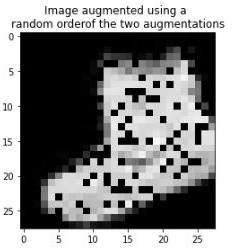
From the preceding image, we can see that the two augmentations are performed on top of the original image (you can observe that the image has been rotated and that dropout has been applied).
Performing data augmentation on a batch of images and the need for collate_fn
We have already seen that it is preferable to perform different augmentations in different iterations on the same image.
If we have an augmentation pipeline defined in the __init__ method, we would only need to perform augmentation once on the input set of images. This means we would not have different augmentations on different iterations.
Similarly, if the augmentation is in the __getitem__ method – which is ideal since we want to perform a different set of augmentations on each image – the major bottleneck is that the augmentation is performed once for each image. It would be much faster if we were to perform augmentation on a batch of images instead of on one image at a time. Let's understand this in detail by looking at two scenarios where we will be working on 32 images:
- Augmenting 32 images, one at a time
- Augmenting 32 images as a batch in one go
To understand the time it takes to augment 32 images in both scenarios, let's leverage the first 32 images in the training images of the Fashion-MNIST dataset:
- Fetch the first 32 images in the training dataset:
from torchvision import datasets
import torch
data_folder = '/content/'
fmnist = datasets.FashionMNIST(data_folder, download=True,
                                                train=True)
tr_images = fmnist.data
tr_targets = fmnist.targets
- Specify the augmentation to be performed on the images:
from imgaug import augmenters as iaa
aug = iaa.Sequential([
              iaa.Affine(translate_px={'x':(-10,10)},
                                        mode='constant'),
            ])
Next, we need to understand how to perform augmentation in the Dataset class. There are two possible ways of augmenting data:
- Augmenting a batch of images, one at a time
- Augmenting all the images in a batch in one go
Let's understand the time it takes to perform both the preceding scenarios:
- Scenario 1: Augmenting 32 images, one at a time:
Calculate the time it takes to augment one image at a time using the augment_image method:
%%time
for i in range(32):
    aug.augment_image(tr_images[i])
It takes ~180 milliseconds to augment for the 32 images.
- Scenario 2: Augmenting 32 images as a batch in one go:
Calculate the time it takes to augment the batch of 32 images in one go using the augment_images method:
%%time
aug.augment_images(tr_images[:32])
It takes ~8 milliseconds to perform augmentation on the batch of images.
However, the traditional Dataset class that we have been working on provides the index of one image at a time in the __getitem__ method. Hence, we need to learn how to use a new function – collate_fn – that enables us to perform manipulation on a batch of images.
- Define the Dataset class, which takes the input images, their classes, and the augmentation object as initializers:
from torch.utils.data import Dataset, DataLoader
class FMNISTDataset(Dataset):
    def __init__(self, x, y, aug=None):
        self.x, self.y = x, y
        self.aug = aug
    def __getitem__(self, ix):
        x, y = self.x[ix], self.y[ix]
        return x, y
    def __len__(self): return len(self.x)
- Define collate_fn, which takes the batch of data as input:
def collate_fn(self, batch):
- Separate the batch of images and their classes into two different variables:
ims, classes = list(zip(*batch))
- Specify that augmentation must be done if the augmentation object is provided. This is useful is we need to perform augmentation on training data but not on validation data:
if self.aug: ims=self.aug.augment_images(images=ims)
In the preceding code, we leveraged the augment_images method so that we can work on a batch of images.
- Create tensors of images, along with scaling data, by dividing the image shape by 255:
        ims = torch.tensor(ims)[:,None,:,:].to(device)/255.
        classes = torch.tensor(classes).to(device)
        return ims, classes
- From now on, to leverage the collate_fn method, we'll use a new argument while creating the DataLoader:
- First, we create the train object:
train = FMNISTDataset(tr_images, tr_targets, aug=aug)
- Next, we define the DataLoader, along with the object's collate_fn method, as follows:
trn_dl = DataLoader(train, batch_size=64,
                    collate_fn=train.collate_fn,shuffle=True)
- Finally, we train the model, as we have been training it so far. By leveraging the collate_fn method, we can train a model faster.
Now that we have a solid understanding of some of the prominent data augmentation techniques we can use, including pixel translation and collate_fn, which allows us to augment a batch of images, let's understand how they can be applied to a batch of data to address image translation issues.
Data augmentation for image translation
Now, we are in a position to train the model with augmented data. Let's create some augmented data and train the model:
- Import the relevant packages and dataset:
from torchvision import datasets
import torch
from torch.utils.data import Dataset, DataLoader
import torch
import torch.nn as nn
import matplotlib.pyplot as plt
%matplotlib inline
import numpy as np

device = 'cuda' if torch.cuda.is_available() else 'cpu'
data_folder = '/content/' # This can be any directory
# you want to download FMNIST to
fmnist = datasets.FashionMNIST(data_folder, download=True,
                                        train=True)
tr_images = fmnist.data
tr_targets = fmnist.targets
val_fmnist=datasets.FashionMNIST(data_folder, download=True,
                                        train=False)
val_images = val_fmnist.data
val_targets = val_fmnist.targets
- Create a class that can perform data augmentation on an image that's translated randomly anywhere between -10 to +10 pixels, either to the left or to the right:
- Define the data augmentation pipeline:
from imgaug import augmenters as iaa
aug = iaa.Sequential([
              iaa.Affine(translate_px={'x':(-10,10)},
                                        mode='constant'),
            ])
- Define the Dataset class:
class FMNISTDataset(Dataset):
    def __init__(self, x, y, aug=None):
        self.x, self.y = x, y
        self.aug = aug
    def __getitem__(self, ix):
        x, y = self.x[ix], self.y[ix]
        return x, y
    def __len__(self): return len(self.x)
    def collate_fn(self, batch):
        'logic to modify a batch of images'
        ims, classes = list(zip(*batch))
        # transform a batch of images at once
        if self.aug: ims=self.aug.augment_images(images=ims)
        ims = torch.tensor(ims)[:,None,:,:].to(device)/255.
        classes = torch.tensor(classes).to(device)
        return ims, classes
In the preceding code, we've leveraged the collate_fn method to specify that we want to perform augmentations on a batch of images.
- Define the model architecture, as we did in the previous section:
from torch.optim import SGD, Adam
def get_model():
    model = nn.Sequential(
                nn.Conv2d(1, 64, kernel_size=3),
                nn.MaxPool2d(2),
                nn.ReLU(),
                nn.Conv2d(64, 128, kernel_size=3),
                nn.MaxPool2d(2),
                nn.ReLU(),
                nn.Flatten(),
                nn.Linear(3200, 256),
                nn.ReLU(),
                nn.Linear(256, 10)
            ).to(device)

    loss_fn = nn.CrossEntropyLoss()
    optimizer = Adam(model.parameters(), lr=1e-3)
    return model, loss_fn, optimizer
- Define the train_batch function in order to train on batches of data:
def train_batch(x, y, model, opt, loss_fn):
    model.train()
    prediction = model(x)
    batch_loss = loss_fn(prediction, y)
    batch_loss.backward()
    optimizer.step()
    optimizer.zero_grad()
    return batch_loss.item()
- Define the get_data function to fetch the training and validation DataLoaders:
def get_data():
    train = FMNISTDataset(tr_images, tr_targets, aug=aug)
    'notice the collate_fn argument'
    trn_dl = DataLoader(train, batch_size=64,
                collate_fn=train.collate_fn, shuffle=True)
    val = FMNISTDataset(val_images, val_targets)
    val_dl = DataLoader(val, batch_size=len(val_images),
                collate_fn=val.collate_fn, shuffle=True)
    return trn_dl, val_dl
- Specify the training and validation DataLoaders and fetch the model object, loss function, and optimizer:
trn_dl, val_dl = get_data()
model, loss_fn, optimizer = get_model()
- Train the model over 5 epochs:
for epoch in range(5):
    for ix, batch in enumerate(iter(trn_dl)):
        x, y = batch
        batch_loss = train_batch(x, y, model, optimizer,
                                            loss_fn)
- Test the model on a translated image, as we did in the previous section:
preds = []
ix = 24300
for px in range(-5,6):
    img = tr_images[ix]/255.
    img = img.view(28, 28)
    img2 = np.roll(img, px, axis=1)
    plt.imshow(img2)
    plt.show()
    img3 = torch.Tensor(img2).view(-1,1,28,28).to(device)
    np_output = model(img3).cpu().detach().numpy()
    preds.append(np.exp(np_output)/np.sum(np.exp(np_output)))
Now, let's plot the variation in the prediction class across different translations:
import seaborn as sns
fig, ax = plt.subplots(1,1, figsize=(12,10))
plt.title('Probability of each class
for various translations')
sns.heatmap(np.array(preds).reshape(11,10), annot=True,
            ax=ax, fmt='.2f', xticklabels=fmnist.classes,
            yticklabels=[str(i)+str(' pixels')
                         for i in range(-5,6)], cmap='gray')
The preceding code results in the following output:

Now, when we predict for various translations of an image, we'll see that the class prediction does not vary, thus ensuring that image translation is taken care of by training our model on augmented, translated images.
So far, we have seen how a CNN model trained with augmented images can predict well on translated images. In the next section, we'll understand what the filters learn, which makes predicting translated images possible.
Visualizing the outcome of feature learning
So far, we have learned about how CNNs help us classify images, even when the objects in the images have been translated. We have also learned that filters play a key role in learning the features of an image, which, in turn, help in classifying the image into the right class. However, we haven't mentioned what the filters learn that makes them powerful.
In this section, we will learn about what these filters learn that enables CNNs to classify an image correctly by classifying a dataset that contains images of X's and O's. We will also examine the fully connected layer (flatten layer) to understand what their activations look like. Let's take a look at what the filters learn:
- Download the dataset:
!wget https://www.dropbox.com/s/5jh4hpuk2gcxaaq/all.zip
!unzip all.zip
Note that the images in the folder are named as follows:

The class of an image can be obtained from the image's name, where the first character of the image's name specifies the class the image belongs to.
- Import the required modules:
import torch
from torch import nn
from torch.utils.data import TensorDataset,Dataset,DataLoader
from torch.optim import SGD, Adam
device = 'cuda' if torch.cuda.is_available() else 'cpu'
from torchvision import datasets
import numpy as np, cv2
import matplotlib.pyplot as plt
%matplotlib inline
from glob import glob
from imgaug import augmenters as iaa
- Define a class that fetches data. Also, ensure that the images have been resized to a shape of 28 x 28, batches have been shaped with three channels, and that the dependent variable is fetched as a numeric value. We'll do this in the following code, one step at a time:
- Define the image augmented method, which resizes the image to a shape of 28 x 28:
tfm = iaa.Sequential(iaa.Resize(28))
- Define a class that takes the folder path as input and loops through the files in that path in the __init__ method:
class XO(Dataset):
    def __init__(self, folder):
        self.files = glob(folder)
- Define the __len__ method, which returns the lengths of the files that are to be considered:
def __len__(self): return len(self.files)
- Define the __getitem__ method, which we use to fetch an index that returns the file present at that index, read the file, and then perform augmentation on the image. We have not used collate_fn here because this is a small dataset and it wouldn't affect the training time significantly:
    def __getitem__(self, ix):
        f = self.files[ix]
        im = tfm.augment_image(cv2.imread(f)[:,:,0])
- Given that each image is of the shape 28 x 28, we'll now create a dummy channel dimension at the beginning of the shape; that is, before the height and width of an image:
im = im[None]
- Now, we can assign the class of each image based on the character post '/' and prior to '@' in the filename:
cl = f.split('/')[-1].split('@')[0] == 'x'
- Finally, we return the image and the corresponding class:
        return torch.tensor(1 - im/255).to(device).float(),
                       torch.tensor([cl]).float().to(device)
- Inspect a sample of the images you've obtained. In the following code, we're extracting the images and their corresponding classes by fetching data from the class we defined previously:
data = XO('/content/all/*')
- Now, we can plot a sample of the images from the dataset we've obtained:
R, C = 7,7
fig, ax = plt.subplots(R, C, figsize=(5,5))
for label_class, plot_row in enumerate(ax):
    for plot_cell in plot_row:
        plot_cell.grid(False); plot_cell.axis('off')
        ix = np.random.choice(1000)
        im, label = data[ix]
        print()
        plot_cell.imshow(im[0].cpu(), cmap='gray')
plt.tight_layout()
The preceding code results in the following output:

- Define the model architecture, loss function, and the optimizer:
from torch.optim import SGD, Adam
def get_model():
    model = nn.Sequential(
                nn.Conv2d(1, 64, kernel_size=3),
                nn.MaxPool2d(2),
                nn.ReLU(),
                nn.Conv2d(64, 128, kernel_size=3),
                nn.MaxPool2d(2),
                nn.ReLU(),
                nn.Flatten(),
                nn.Linear(3200, 256),
                nn.ReLU(),
                nn.Linear(256, 1),
                nn.Sigmoid()
            ).to(device)

    loss_fn = nn.BCELoss()
    optimizer = Adam(model.parameters(), lr=1e-3)
    return model, loss_fn, optimizer
Note that the loss function is binary cross-entropy loss (nn.BCELoss()) since the output provided is from a binary class. A summary of the preceding model can be obtained as follows:
!pip install torch_summary
from torchsummary import summary
model, loss_fn, optimizer = get_model()
summary(model, torch.zeros(1,1,28,28));
This results in the following output:

- Define a function for training on batches that takes images and their classes as input and returns their loss values and accuracy after backpropagation has been performed on top of the given batch of data:
def train_batch(x, y, model, opt, loss_fn):
    model.train()
    prediction = model(x)
    is_correct = (prediction > 0.5) == y
    batch_loss = loss_fn(prediction, y)
    batch_loss.backward()
    optimizer.step()
    optimizer.zero_grad()
    return batch_loss.item(), is_correct[0]
- Define a DataLoader where the input is the Dataset class:
trn_dl = DataLoader(XO('/content/all/*'), batch_size=32,
drop_last=True)- Initialize the model:
model, loss_fn, optimizer = get_model()- Train the model over 5 epochs:
for epoch in range(5):
    for ix, batch in enumerate(iter(trn_dl)):
        x, y = batch
        batch_loss = train_batch(x, y, model, optimizer,
                                        loss_fn)
- Fetch an image to check what the filters learn about the image:
im, c = trn_dl.dataset[2]
plt.imshow(im[0].cpu())
plt.show()
This results in the following output:

- Pass the image through the trained model and fetch the output of the first layer. Then, store it in the intermediate_output variable:
first_layer = nn.Sequential(*list(model.children())[:1])
intermediate_output = first_layer(im[None])[0].detach()
- Plot the output of the 64 filters. Each channel in intermediate_output is the output of the convolution for each filter:
fig, ax = plt.subplots(8, 8, figsize=(10,10))
for ix, axis in enumerate(ax.flat):
    axis.set_title('Filter: '+str(ix))
    axis.imshow(intermediate_output[ix].cpu())
plt.tight_layout()
plt.show()
This results in the following output:
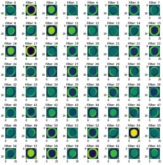
In the preceding output, notice that certain filters, such as filters 0, 4, 6, and 7, learn about the edges present in the network, while other filters, such as filter 54, learned to invert the image.
- Pass multiple O images and inspect the output of the fourth filter across the images (we are only using the fourth filter for illustration purposes; you can choose a different filter if you wish):
- Fetch multiple O images from the data:
x, y = next(iter(trn_dl))
x2 = x[y==0]
- Reshape x2 so that it has a proper input shape for a CNN model; that is, batch size x channels x height x width:
x2 = x2.view(-1,1,28,28)
- Define a variable that stores the model until the first layer:
first_layer = nn.Sequential(*list(model.children())[:1])
- Extract the output of passing the O images (x2) through the model until the first layer (first_layer), as defined previously:
first_layer_output = first_layer(x2).detach()
- Plot the output of passing multiple images through the first_layer model:
n = 4
fig, ax = plt.subplots(n, n, figsize=(10,10))
for ix, axis in enumerate(ax.flat):
    axis.imshow(first_layer_output[ix,4,:,:].cpu())
    axis.set_title(str(ix))
plt.tight_layout()
plt.show()
The preceding code results in the following output:

- Now, let's create another model that extracts layers until the second convolution layer (that is, until the four layers defined in the preceding model) and then extracts the output of passing the original O image. We will then plot the output of convolving the filters in the second layer with the input O image:
second_layer = nn.Sequential(*list(model.children())[:4])
second_intermediate_output=second_layer(im[None])[0].detach()
- Plot the output of convolving the filters with the respective image:
fig, ax = plt.subplots(11, 11, figsize=(10,10))
for ix, axis in enumerate(ax.flat):
    axis.imshow(second_intermediate_output[ix].cpu())
    axis.set_title(str(ix))
plt.tight_layout()
plt.show()
The preceding code results in the following output:

Now, let's use the 34th filter's output in the preceding image as an example. When we pass multiple O images through filter 34, we should see similar activations across images. Let's test this, as follows:
second_layer = nn.Sequential(*list(model.children())[:4])
second_intermediate_output = second_layer(x2).detach()
fig, ax = plt.subplots(4, 4, figsize=(10,10))
for ix, axis in enumerate(ax.flat):
    axis.imshow(second_intermediate_output[ix,34,:,:].cpu())
    axis.set_title(str(ix))
plt.tight_layout()
plt.show()
The preceding code results in the following output:

Note that, even here, the activations of the 34th filter on different images are similar in that the left half of O was activating the filter.
- Plot the activations of a fully connected layer, as follows:
- First, fetch a larger sample of images:
custom_dl= DataLoader(XO('/content/all/*'),batch_size=2498,
                       drop_last=True)
- Next, choose only the O images from the dataset and then reshape them so that they can be passed as input to our CNN model:
x, y = next(iter(custom_dl))
x2 = x[y==0]
x2 = x2.view(len(x2),1,28,28)
- Fetch the flatten (fully connected) layer and pass thee preceding images through the model until they reach the flattened layer:
flatten_layer = nn.Sequential(*list(model.children())[:7])
flatten_layer_output = flatten_layer(x2).detach()
- Plot the flattened layer:
plt.figure(figsize=(100,10))
plt.imshow(flatten_layer_output.cpu())
The preceding code results in the following output:

Note that the shape of the output is 1245 x 3200 since there are 1,245 O images in our dataset and there are 3,200 dimensions for each image in the flattening layer.
It's also interesting to note that certain values in the fully connected layer are highlighted when the input is O (here, we can see white lines, where each dot represents an activation value greater than zero).
Now that we have learned how CNNs work and how filters aid in this process, we will apply this so that we can classify images of cats and dogs.
Building a CNN for classifying real-world images
So far, we have learned how to perform image classification on the Fashion-MNIST dataset. In this section, we'll do the same for a more real-world scenario, where the task is to classify images containing cats or dogs. We will also learn about how the accuracy of the dataset varies when we change the number of images available for training.
We will be working on a dataset available in Kaggle: https://www.kaggle.com/tongpython/cat-and-dog.
- Import the necessary packages:
import torchvision
import torch.nn as nn
import torch
import torch.nn.functional as F
from torchvision import transforms,models,datasets
from PIL import Image
from torch import optim
device = 'cuda' if torch.cuda.is_available() else 'cpu'
import cv2, glob, numpy as np, pandas as pd
import matplotlib.pyplot as plt
%matplotlib inline
from glob import glob
!pip install torch_summary
- Download the dataset, as follows:
- Here, we must download the dataset that's available in the colab environment. First, however, we must upload our Kaggle authentication file:
!pip install -q kaggle
from google.colab import files
files.upload()
- Next, specify that we're moving to the Kaggle folder and copy the kaggle.json file to it:
!mkdir -p ~/.kaggle
!cp kaggle.json ~/.kaggle/
!ls ~/.kaggle
!chmod 600 /root/.kaggle/kaggle.json
- Finally, download the cats and dogs dataset and unzip it:
!kaggle datasets download -d tongpython/cat-and-dog
!unzip cat-and-dog.zip
- Provide the training and test dataset folders:
train_data_dir = '/content/training_set/training_set'
test_data_dir = '/content/test_set/test_set'
- Build a class that fetches data from the preceding folders. Then, based on the directory the image corresponds to, provide a label of 1 for "dog" images and a label of 0 for "cat" images. Furthermore, ensure that the fetched image has been normalized to a scale between 0 and 1 and permute it so that channels are provided first (as PyTorch models expect to have channels specified first, before the height and width of the image).
- Define the __init__ method, which takes a folder as input and stores the file paths (image paths) corresponding to the images in the cats and dogs folders in separate objects, post concatenating the file paths into a single list:
from torch.utils.data import DataLoader, Dataset
class cats_dogs(Dataset):
    def __init__(self, folder):
        cats = glob(folder+'/cats/*.jpg')
        dogs = glob(folder+'/dogs/*.jpg')
        self.fpaths = cats + dogs
- Next, randomize the file paths and create target variables based on the folder corresponding to these file paths:
        from random import shuffle, seed; seed(10);
        shuffle(self.fpaths)
        self.targets=[fpath.split('/')[-1].startswith('dog')
                      for fpath in self.fpaths] # dog=1
- Define the __len__ method, which corresponds to the self class:
def __len__(self): return len(self.fpaths)
- Define the __getitem__ method, which we use to specify a random file path from the list of file paths, read the image, and resize all the images so that they're 224 x 224 in size. Given that our CNN expects the inputs from the channel to be specified first for each image, we will permute the resized image so that channels are provided first before we return the scaled image and the corresponding target value:
    def __getitem__(self, ix):
        f = self.fpaths[ix]
        target = self.targets[ix]
        im = (cv2.imread(f)[:,:,::-1])
        im = cv2.resize(im, (224,224))
        return torch.tensor(im/255).permute(2,0,1)
                    .to(device).float(),
               torch.tensor([target])
                    .float().to(device)
- Inspect a random image:
data = cats_dogs(train_data_dir)
im, label = data[200]
We need to permute the image we've obtained to our channels last. This is because matplotlib expects an image to have the channels specified after the height and width of the image has been provided:
plt.imshow(im.permute(1,2,0).cpu())
print(label)
This results in the following output:

- Define a model, loss function, and optimizer, as follows:
- First, we must define the conv_layer function, where we perform convolution, ReLU activation, batch normalization, and max pooling in that order. This method will be reused in the final model, which we will define in the next step:
def conv_layer(ni,no,kernel_size,stride=1):
    return nn.Sequential(
        nn.Conv2d(ni, no, kernel_size, stride),
        nn.ReLU(),
        nn.BatchNorm2d(no),
        nn.MaxPool2d(2)
    )
In the preceding code, we are taking the number of input channels (ni), number of output channels (no), kernel_size, and the stride of filters as input for the conv_layer function.
- Define the get_model function, which performs multiple convolutions and pooling operations (by calling the conv_layer method), flattens the output, and connects a hidden layer to it prior to connecting to the output layer:
def get_model():
    model = nn.Sequential(
              conv_layer(3, 64, 3),
              conv_layer(64, 512, 3),
              conv_layer(512, 512, 3),
              conv_layer(512, 512, 3),
              conv_layer(512, 512, 3),
              conv_layer(512, 512, 3),
              nn.Flatten(),
              nn.Linear(512, 1),
              nn.Sigmoid(),
            ).to(device)
    loss_fn = nn.BCELoss()
    optimizer = torch.optim.Adam(model.parameters(), lr= 1e-3)
    return model, loss_fn, optimizer
- Now, we must call the get_model function to fetch the model, loss function (loss_fn), and optimizer and then summarize the model using the summary method that we imported from the torchsummary package:
from torchsummary import summary
model, loss_fn, optimizer = get_model()
summary(model, torch.zeros(1,3, 224, 224));
The preceding code results in the following output:

- Create the get_data function, which creates an object of the cats_dogs class and creates a DataLoader with a batch_size of 32 for both the training and validation folders:
def get_data():
    train = cats_dogs(train_data_dir)
    trn_dl = DataLoader(train, batch_size=32, shuffle=True,
                            drop_last = True)
    val = cats_dogs(test_data_dir)
    val_dl = DataLoader(val, batch_size=32, shuffle=True,
                            drop_last = True)
    return trn_dl, val_dl
In the preceding code, we are ignoring the last batch of data by specifying that drop_last = True. We're doing this because the last batch might not be the same size as the other batches.
- Define the function that will train the model on a batch of data, as we've done in previous sections:
def train_batch(x, y, model, opt, loss_fn):
    model.train()
    prediction = model(x)
    batch_loss = loss_fn(prediction, y)
    batch_loss.backward()
    optimizer.step()
    optimizer.zero_grad()
    return batch_loss.item()
- Define the functions for calculating accuracy and validation loss, as we've done in previous sections:
- Define the accuracy function:
@torch.no_grad()
def accuracy(x, y, model):
    prediction = model(x)
    is_correct = (prediction > 0.5) == y
    return is_correct.cpu().numpy().tolist()
Note that the preceding code for accuracy calculation is different from the code in the Fashion-MNIST classification because the current model (cats versus dogs classification) is being built for binary classification, while the Fashion-MNIST model was built for multi-class classification.
- Define the validation loss calculation function:
@torch.no_grad()
def val_loss(x, y, model):
    prediction = model(x)
    val_loss = loss_fn(prediction, y)
    return val_loss.item()
- Train the model for 5 epochs and check the accuracy of the test data at the end of each epoch, as we've done in previous sections:
- Define the model and fetch the required DataLoaders:
trn_dl, val_dl = get_data()
model, loss_fn, optimizer = get_model()
- Train the model over increasing epochs:
train_losses, train_accuracies = [], []
val_losses, val_accuracies = [], []
for epoch in range(5):
    train_epoch_losses, train_epoch_accuracies = [], []
    val_epoch_accuracies = []
    for ix, batch in enumerate(iter(trn_dl)):
        x, y = batch
        batch_loss = train_batch(x, y, model, optimizer,
                                            loss_fn)
        train_epoch_losses.append(batch_loss)
    train_epoch_loss = np.array(train_epoch_losses).mean()

    for ix, batch in enumerate(iter(trn_dl)):
        x, y = batch
        is_correct = accuracy(x, y, model)
        train_epoch_accuracies.extend(is_correct)
    train_epoch_accuracy = np.mean(train_epoch_accuracies)

    for ix, batch in enumerate(iter(val_dl)):
        x, y = batch
        val_is_correct = accuracy(x, y, model)
        val_epoch_accuracies.extend(val_is_correct)
    val_epoch_accuracy = np.mean(val_epoch_accuracies)

    train_losses.append(train_epoch_loss)
    train_accuracies.append(train_epoch_accuracy)
    val_accuracies.append(val_epoch_accuracy)
- Plot the variation of the training and validation accuracies over increasing epochs:
epochs = np.arange(5)+1
import matplotlib.ticker as mtick
import matplotlib.pyplot as plt
import matplotlib.ticker as mticker
%matplotlib inline
plt.plot(epochs, train_accuracies, 'bo',
         label='Training accuracy')
plt.plot(epochs, val_accuracies, 'r',
         label='Validation accuracy')
plt.gca().xaxis.set_major_locator(mticker.MultipleLocator(1))
plt.title('Training and validation accuracy
with 4K data points used for training')
plt.xlabel('Epochs')
plt.ylabel('Accuracy')
plt.gca().set_yticklabels(['{:.0f}%'.format(x*100)
                           for x in plt.gca().get_yticks()])
plt.legend()
plt.grid('off')
plt.show()
The preceding code results in the following output:

Note that the classification accuracy at the end of 5 epochs is ~86%.
So far, the training we've done has been based on ~8K examples, where 4K examples have been from the cat class and the rest have been from the dog class. In the next section, we will learn about what impact having a reduced number of training examples has on each class when it comes to the classification accuracy of the test dataset.
Impact on the number of images used for training
We know that, generally, the more training examples we use, the better our classification accuracy is. In this section, we will learn what impact using different numbers of available images has on training accuracy by artificially reducing the number of images available for training and then testing the model's accuracy when classifying the test dataset.
Here, we only want to have 500 data points for each class in the training dataset. We can do this by limiting the number of files to only the first 500 image paths in each folder in the __init__ method and ensuring the rest remain as they were in the previous section:
    def __init__(self, folder):
        cats = glob(folder+'/cats/*.jpg')
        dogs = glob(folder+'/dogs/*.jpg')
        self.fpaths = cats[:500] + dogs[:500]
        from random import shuffle, seed; seed(10);
            shuffle(self.fpaths)
        self.targets = [fpath.split('/')[-1].startswith('dog')
                        for fpath in self.fpaths]
In the preceding code, the only difference from the initialization we performed in the previous section is in self.paths, where we are now limiting the number of file paths to be considered in each folder to only the first 500.
Now, once we execute the rest of the code, as we did in the previous section, the accuracy of the model that's been built on 1,000 images (500 of each class) in the test dataset will be as follows:

Here, we can see that because we had fewer examples of images in training, the accuracy of the test dataset reduced considerably; that is, down to ~66%.
Now, let's see how the number of training data points impacts the accuracy of the test dataset by varying the number of available training examples that will be used to train the model (where we build a model for each scenario).
We'll use the same code we used for the 500 data point training example but will vary the number of available images (to 2K, 4K, and 8K total data points, respectively). For brevity, we will only look at the output of running the model on a varying number of images available for training. This results in the following output:

As you can see, the more training data that's available, the higher the accuracy of the model on test data. However, we might not have a large enough amount of training data in every scenario that we encounter. The next chapter, which will cover transfer learning, will address this problem by walking you through various techniques you can use to attain high accuracy, even on a small amount of training data.
Summary
Traditional neural networks fail when new images that are very similar to previously seen images that have been translated are fed as input to the model. Convolutional neural networks play a key role in addressing this shortcoming. This is enabled through the various mechanisms that are present in CNNs, including filters, strides, and pooling. Initially, we built a toy example to learn about how CNNs work. Then, we learned about how data augmentation helps in increasing the accuracy of the model by creating translated augmentations on top of the original image. After that, we learned about what different filters learn in the feature learning process so that we could implement a CNN to classify images.
Finally, we saw the impact that differing amounts of training data have on the accuracy of test data. Here, we saw that the more training data that is available, the better the accuracy of the test data. In the next chapter, we will learn about how to leverage various transfer learning techniques to increase the accuracy of the test dataset, even when we have just a small amount of training data.
Questions
- Why is the prediction on a translated image low when using traditional neural networks?
- How is convolution done?
- How are optimal weight values in a filter identified?
- How does the combination of convolution and pooling help in addressing the issue of image translation?
- What do the filters in layers closer to the input layer learn?
- What functionality does pooling have that helps in building a model?
- Why can't we take an input image, flatten it (as we did on the Fashion-MNIST dataset), and then train a model for real-world images?
- How does data augmentation help in improving image translation?
- In what scenario do we leverage collate_fn for DataLoaders?
- What impact does varying the number of training data points have on the classification accuracy of the validation dataset?