In the previous chapter, we learned about how to combine NLP techniques (LSTM and transformer) with computer vision-based techniques. In this chapter, we will learn how to combine reinforcement learning-based techniques (primarily deep Q-learning) with computer vision-based techniques.
We will start by learning about the basics of reinforcement learning and then about the terminology associated with identifying how to calculate the value (Q-value) associated with taking an action in a given state. Next, we will learn about filling a Q-table, which helps in identifying the value associated with various actions in a given state. Furthermore, we will learn about identifying the Q-values of various actions in scenarios where coming up with a Q-table is infeasible due to a high number of possible states; we'll do this using Deep Q-Network. This is where we will understand how to leverage neural networks in combination with reinforcement learning. Next, we will learn about scenarios where the Deep Q-Network model does not work and address this by using the Deep Q-Network alongside the fixed targets model. Here, we will play a video game known as Pong by leveraging CNN in conjunction with reinforcement learning. Finally, we will leverage what we've learned to build an agent that can drive a car autonomously in a simulated environment – CARLA.
In summary, in this chapter, we will cover the following topics:
- Learning the basics of reinforcement learning
- Implementing Q-learning
- Implementing deep Q-learning
- Implementing deep Q-learning with fixed targets
- Implementing an agent to perform autonomous driving
Learning the basics of reinforcement learning
Reinforcement learning (RL) is an area of machine learning concerned with how software agents ought to take actions in a given state of an environment to maximize the notion of cumulative reward.
To understand how RL helps, let's consider a simple scenario. Imagine that you are playing chess against a computer (in our case, the computer is an agent that has learned/is learning how to play chess). The setup (rules) of the game constitutes the environment. Furthermore, as we make a move (take an action), the state of the board (the location of various pieces on the chessboard) changes. At the end of the game, depending on the result, the agent gets a reward. The objective of the agent is to maximize the reward.
If the machine (agent1) is playing against a human, the number of games that it can play is finite (depending on the number of games the human can play). This might create a bottleneck for the agent to learn well. However, what if agent1 (the agent that is learning the game) can play against agent2 (agent2 could be another agent that is learning chess or it could be a piece of chess software that has been pre-programmed to play the game well)? Theoretically, the agents can play infinite games with each other, which results in maximizing the opportunity to learn to play the game well. This way, by playing multiple games with each other, the learning agent is likely to learn how to address the different scenarios/states of the game well.
Let's understand the process that the learning agent will follow to learn well:
- Initially, the agent takes a random action in a given state.
- The agent stores the action it has taken in various states within a game in memory.
- Then, the agent associates the result of the action in various states with a reward.
- After playing multiple games, the agent can correlate the action in a state to a potential reward by replaying its experiences.
Next comes the question of quantifying the value that corresponds to taking an action in a given state. We'll learn how to calculate this in the next section.
Calculating the state value
To understand how to quantify the value of a state, let's use a simple scenario where we will define the environment and objective as follows:

The environment is a grid with two rows and three columns. The agent starts at the Start cell and it achieves its objective (rewarded with a score of +1) if the agent reaches the bottom-right grid cell. The agent does not get a reward if it goes to any other cell. The agent can take an action by going to the right, left, bottom, or up, depending on the feasibility of the action (the agent can go to the right or to the bottom in the start grid cell, for example). The reward of reaching any of the remaining cells other than the bottom-right cell is 0.
By using this information, let's calculate the value of a cell (the state that the agent is in, in a given snapshot). Given that some energy is spent moving from one cell to another, we discount the value of reaching a cell by a factor of γ, where γ takes care of the energy that's spent in moving from one cell to another. Furthermore, the introduction of γ results in the agent learning to play well sooner. With this, let's formalize the Bellman equation, which helps in calculating the value of a cell:

With the preceding equation in place, let's calculate the values of all cells (once the optimal actions in a state have been identified) with the value of γ being 0.9 (the typical value of γ is between 0.9 and 0.99):

From the preceding calculations, we can understand how to calculate the values in a given state (cell), when given the optimal actions in that state. These are as follows for our simplistic scenario of reaching the terminal state:

With the values in place, we expect the agent to follow a path of increasing value.
Now that we understand how to calculate the state value, in the next section, we will understand how to calculate the value associated with a state-action combination.
Calculating the state-action value
In the previous section, we provided a scenario where we already know that the agent is taking optimal actions (which is not realistic). In this section, we will look at a scenario where we can identify the value that corresponds to a state-action combination.
In the following image, each sub-cell within a cell represents the value of taking an action in the cell. Initially, the cell values for various actions are as follows:
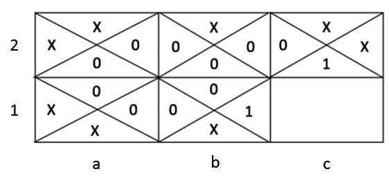
Note that, in the preceding image, cell b1 (2nd row and 2nd column) will have a value of 1 if the agent moves right from the cell (as it corresponds to the terminal cell); the other actions result in a value of 0. X represents that the action is not possible and hence no value is associated with it.
Over four iterations (steps), the updated cell values for the actions in the given state are as follows:

This would then go through multiple iterations to provide the optimal action that maximizes value at each cell.
Let's understand how to obtain the cell values in the second table (Iteration 2 in the preceding image). Let's narrow this down to 0.3, which was obtained by taking the downward action when present in the 1st row and 2nd column of the second table. When the agent takes the downward action, there is a 1/3 chance of it taking the optimal action in the next state. Hence, the value of taking a downward action is as follows:

In a similar manner, we can obtain the values of taking different possible actions in different cells.
Now that we know how the values of various actions in a given state are calculated, in the next section, we will learn about Q-learning and how we can leverage it, along with the Gym environment, so that it can play various games.
Implementing Q-learning
In the previous section, we manually calculated the state-action values for all combinations. Technically, now that we have calculated the various state-action values we need, we can now identify the action that will be taken in every state. However, in the case of a more complex scenario – for example, when playing video games – it gets tricky to fetch state information. OpenAI's Gym environment comes in handy in this scenario. It contains a pre-defined environment for the game we're playing. Here, it fetches the next state information, given an action that's been taken in the current state. So far, we have considered the scenario of choosing the most optimal path. However, there can be scenarios where we are stuck at the local minima.
In this section, we will learn about Q-learning, which helps with calculating the value associated with the action in a state, as well as about leveraging the Gym environment so that we can play various games. For now, we'll take a look at a simple game called Frozen Lake. We'll also take a look at exploration-exploitation, which helps us avoid getting stuck at the local minima. However, before we do that, we will learn about the Q-value.
Q-value
The Q in Q-learning or Q-value represents the quality of an action. Let's learn how to calculate it:

We already know that we must keep updating the state-action value of a given state until it is saturated. Hence, we'll modify the preceding formula like so:

In the preceding equation, we replace 1 with the learning rate so that we can update the value of the action that's taken in a state more gradually:

With this formal definition of Q-value in place, in the next section, we'll learn about the Gym environment and how it helps us fetch the Q-table (which stores information about the values of various actions that have been taken at various states) and thus come up with the optimal actions in a state.
Understanding the Gym environment
In this section, we will explore the Gym environment and the various functionalities present in it while playing the Frozen Lake game present in the Gym environment:
- Import the relevant packages:
import numpy as np
import gym
import random
- Print the various environments present in the Gym environment:
from gym import envs
print(envs.registry.all())
The preceding code prints a dictionary containing all the games available within Gym.
- Create an environment for the chosen game:
env = gym.make('FrozenLake-v0', is_slippery=False)- Inspect the created environment:
env.render()
The preceding code results in the following output:

In the preceding image, the agent starts at S. Here, F specifies that the cell is frozen, while H specifies that the cell has a hole in it. The agent gets a reward of 0 if it goes to cell H and the game is terminated. The objective of the game is for the agent to reach G.
- Print the size of the observation space (number of states) in the game:
env.observation_space.n
The preceding code gives us an output of 16. This represents the 16 cells that the game has.
- Print the number of possible actions:
env.action_space.n
The preceding code results in a value of 4, which represents the four possible actions that can be taken.
- Sample a random action at a given state:
env.action_space.sample()
.sample() specifies that we fetch one of the possible four actions in a given state. The scalar corresponding to each action can be associated with the name of the action. We can do this by inspecting the code in GitHub: https://github.com/openai/gym/blob/master/gym/envs/toy_text/frozen_lake.py.
- Reset the environment to its original state:
env.reset()
- Take (step) an action:
env.step(env.action_space.sample())
The preceding code fetches the next state, the reward, the flag that states whether the game was completed, and additional information. We can execute the game with .step since the environment readily provides the next state when it's given a step with an action.
These steps form the basis for us to build a Q-table that dictates the optimal action to be taken in each state. We'll do this in the next section.
Building a Q-table
In the previous section, we learned how to calculate Q-values for various state-action pairs manually. In this section, we will leverage the Gym environment and the various modules associated with it to populate the Q-table – where rows represent the states that an agent can be in and columns represent the actions the agent can take. The values of the Q-table represent the Q-values of taking an action in a given state.
We can populate the values of the Q-table using the following strategy:
- Initialize the game environment and the Q-table with zeros.
- Take a random action and fetch the next state, reward, the flag stating whether the game was completed, and additional information.
- Update the Q-value using the Bellman equation we defined earlier.
- Repeat steps 2 and 3 so that there's a maximum of 50 steps in an episode.
- Repeat steps 2, 3, and 4 over multiple episodes.
Let's code up the preceding strategy:
- Initialize the game environment:
import numpy as np
import gym
import random
env = gym.make('FrozenLake-v0', is_slippery=False)
- Initialize the Q-table with zeros:
action_size=env.action_space.n
state_size=env.observation_space.n
qtable=np.zeros((state_size,action_size))
The preceding code checks the possible actions and states that can be used to build a Q-table. The Q-table's dimension should be the number of states multiplied by the number of actions.
- Play multiple episodes while taking a random action. Here, we reset the environment at the end of every episode:
episode_rewards = []
for i in range(10000):
    state=env.reset()
- Take a maximum of 50 steps per episode:
    total_rewards = 0
    for step in range(50):
We are considering a maximum of 50 steps per episode as it's possible for the agent to keep oscillating between two states forever (think of left and right actions being performed consecutively forever). Thus, we need to specify the maximum number of steps an agent can take.
- Sample a random action and take (step) it:
        action=env.action_space.sample()
        new_state,reward,done,info=env.step(action)
- Update the Q-value that corresponds to the state and the action:
qtable[state,action]+=0.1*(reward+0.9*np.max(
                            qtable[new_state,:])
                           -qtable[state,action])
In the preceding code, we specified that the learning rate is 0.1 and that were are updating the Q-value of a state-action combination by taking the maximum Q-value of the next state (np.max(qtable[new_state,:])) into consideration.
- Update the state value to new_state, which we obtained previously, and accumulate reward into total_rewards:
        state=new_state
        total_rewards+=reward
- Place the rewards in a list (episode_rewards) and print the Q-table (qtable):
    episode_rewards.append(total_rewards)
print(qtable)
The preceding code fetches the Q-values of various actions in a state:

We will learn about how the obtained Q-table is leveraged in the next section.
So far, we have kept taking a random action every time. However, in a realistic scenario, once we have learned that certain actions can't be taken in certain states and vice versa, we don't need to take a random action anymore. The concept of exploration-exploitation comes in handy in such a scenario.
Leveraging exploration-exploitation
In the previous section, we explored the possible actions we can take in a given space. In this section, we will learn about the concept of exploration-exploitation, which can be described as follows:
- Exploration is a strategy where we learn what needs to be done (what action to take) in a given state.
- Exploitation is a strategy where we leverage what has already been learned; that is, which action to take in a given state.
During the initial stages, it is ideal to have a high amount of exploration as the agent won't know what optimal actions to take initially. Through the episodes, as the agent learns the Q-values of various state-action combinations over time, we must leverage exploitation to perform the action that leads to a high reward.
With this intuition in place, let's modify the Q-value calculation that we built in the previous section so that it includes exploration and exploitation:
episode_rewards = []
epsilon=1
max_epsilon=1
min_epsilon=0.01
decay_rate=0.005
for episode in range(1000):
    state=env.reset()
    total_rewards = 0
    for step in range(50):
        exp_exp_tradeoff=random.uniform(0,1)
        ## Exploitation:
        if exp_exp_tradeoff>epsilon:
            action=np.argmax(qtable[state,:])
        else:
            ## Exploration
            action=env.action_space.sample()
        new_state,reward,done,info=env.step(action)
        qtable[state,action]+=0.9*(reward+0.9*np.max(
                                  qtable[new_state,:])
                                   -qtable[state,action])
        state=new_state
        total_rewards+=reward
    episode_rewards.append(total_rewards)
    epsilon=min_epsilon+(max_epsilon-min_epsilon)
                            *np.exp(decay_rate*episode)
print(qtable)
The bold lines in the preceding code are what's been added to the code that was shown in the previous section. Within this code, we are specifying that, over increasing episodes, we perform more exploitation than exploration.
Once we've obtained the Q-table, we can leverage it to identify the steps that the agent needs to take to reach its destination:
env.reset()
for episode in range(1):
    state=env.reset()
    step=0
    done=False
    print("-----------------------")
    print("Episode",episode)
    for step in range(50):
        env.render()
        action=np.argmax(qtable[state,:])
        print(action)
        new_state,reward,done,info=env.step(action)
        if done:
            print("Number of Steps",step+1)
            break
        state=new_state
env.close()
In the preceding code, we are fetching the current state that the agent is in, identifying the action that results in a maximum value in the given state-action combination, taking the action (step) to fetch the new_state object that the agent would be in, and repeating these steps until the game is complete (terminated).
The preceding code results in the following output:

Note that this is a simplified example since the state spaces are discrete, resulting in us building a Q-table. What if the state spaces are continuous (for example, the state space is a snapshot image of a game's current state)? Building a Q-table becomes very difficult (as the number of possible states is very large). Deep Q-learning comes in handy in such a scenario. We'll learn about this in the next section.
Implementing deep Q-learning
So far, we have learned how to build a Q-table, which provides values that correspond to a given state-action combination by replaying a game – in this case, the Frozen Lake game – over multiple episodes. However, when the state spaces are continuous (such as a snapshot of a game of Pong), the number of possible state spaces becomes huge. We will address this in this section, as well as the ones to follow, using deep Q-learning. In this section, we will learn how to estimate the Q-value of a state-action combination without a Q-table by using a neural network – hence the term deep Q-learning.
Compared to a Q-table, deep Q-learning leverages a neural network to map any given state-action (where the state can be continuous or discrete) combination to Q-values.
For this exercise, we will work on the CartPole environment in Gym. Here, our task is to balance the CartPole for as long as possible. The following image shows what the CartPole environment looks like:

Note that the pole shifts to the left when the cart moves to the right and vice versa. Each state within this environment is defined using four observations, whose names and minimum and maximum values are as follows:
| Observation | Minimum Value | Maximum Value |
| Cart position | -2.4 | 2.4 |
| Cart velocity | -inf | inf |
| Pole angle | -41.8° | 41.8° |
| Pole velocity at the tip | -inf | inf |
Note that all the observations that represent a state have continuous values.
At a high level, deep Q-learning for the game of CartPole balancing works as follows:
- Fetch the input values (image of the game/metadata of the game).
- Pass the input values through a network that has as many outputs as there are possible actions.
- The output layers predict the action values that correspond to taking an action in a given state.
A high-level overview of the network architecture is as follows:

In the preceding image, the network architecture uses the state (four observations) as input and the Q-value of taking left and right actions in the current state as output. We train the neural network as follows:
- During the exploration phase, we perform a random action that has the highest value in the output layer.
- Then, we store the action, the next state, the reward, and the flag stating whether the game was complete in memory.
- In a given state, if the game is not complete, the Q-value of taking an action in a given state will be calculated; that is, reward + discount factor x maximum possible Q-value of all actions in the next state.
- The Q-values of the current state-action combinations remain unchanged except for the action that is taken in step 2.
- Perform steps 1 to 4 multiple times and store the experiences.
- Fit a model that takes the state as input and the action values as the expected outputs (from memory and replay experience) and minimize the MSE loss.
- Repeat the preceding steps over multiple episodes while decreasing the exploration rate.
With the preceding strategy in place, let's code up deep Q-learning so that we can perform CartPole balancing:
- Import the relevant packages:
import gym
import numpy as np
import cv2
from collections import deque
import torch
import torch.nn as nn
import torch.nn.functional as F
import random
from collections import namedtuple, deque
import torch.optim as optim
device = 'cuda' if torch.cuda.is_available() else 'cpu'
- Define the environment:
env = gym.make('CartPole-v1')
- Define the network architecture:
class DQNetwork(nn.Module):
    def __init__(self, state_size, action_size):
        super(DQNetwork, self).__init__()

        self.fc1 = nn.Linear(state_size, 24)
        self.fc2 = nn.Linear(24, 24)
        self.fc3 = nn.Linear(24, action_size)

    def forward(self, state):
        x = F.relu(self.fc1(state))
        x = F.relu(self.fc2(x))
        x = self.fc3(x)
        return x
Note that the architecture is fairly simple since it only contains 24 units in the two hidden layers. The output layer contains as many units as there are possible actions.
- Define the Agent class, as follows:
- Define the __init__ method with the various parameters, network, and experience defined:
class Agent():
    def __init__(self, state_size, action_size):

        self.state_size = state_size
        self.action_size = action_size
        self.seed = random.seed(0)

        ## hyperparameters
        self.buffer_size = 2000
        self.batch_size = 64
        self.gamma = 0.99
        self.lr = 0.0025
        self.update_every = 4

        # Q-Network
        self.local = DQNetwork(state_size, action_size)
                                        .to(device)
        self.optimizer=optim.Adam(self.local.parameters(),
                                        lr=self.lr)

        # Replay memory
        self.memory = deque(maxlen=self.buffer_size)
        self.experience = namedtuple("Experience",
                            field_names=["state", "action",
                             "reward", "next_state", "done"])
        self.t_step = 0
- Define the step function, which fetches data from memory and fits it to the model by calling the learn function:
    def step(self, state, action, reward, next_state, done):
        # Save experience in replay memory
        self.memory.append(self.experience(state, action,
                                    reward, next_state, done))
        # Learn every update_every time steps.
        self.t_step = (self.t_step + 1) % self.update_every
        if self.t_step == 0:
        # If enough samples are available in memory,
        # get random subset and learn
            if len(self.memory) > self.batch_size:
                experiences = self.sample_experiences()
                self.learn(experiences, self.gamma)
- Define the act function, which predicts an action, given a state:
    def act(self, state, eps=0.):
        # Epsilon-greedy action selection
        if random.random() > eps:
            state = torch.from_numpy(state).float()
                         .unsqueeze(0).to(device)
            self.local.eval()
            with torch.no_grad():
                action_values = self.local(state)
            self.local.train()
            return np.argmax(action_values.cpu().data.numpy())
        else:
            return random.choice(np.arange(self.action_size))
Note that in the preceding code, we are performing exploration-exploitation while determining the action to take.
- Define the learn function, which fits the model so that it predicts action values when given a state:
    def learn(self, experiences, gamma):
        states,actions,rewards,next_states,dones= experiences
        # Get expected Q values from local model
        Q_expected = self.local(states).gather(1, actions)

        # Get max predicted Q values (for next states)
        # from local model
        Q_targets_next = self.local(next_states).detach()
                             .max(1)[0].unsqueeze(1)
        # Compute Q targets for current states
        Q_targets = rewards+(gamma*Q_targets_next*(1-dones))

        # Compute loss
        loss = F.mse_loss(Q_expected, Q_targets)

        # Minimize the loss
        self.optimizer.zero_grad()
        loss.backward()
        self.optimizer.step()
In the preceding code, we are fetching the sampled experiences and predicting the Q-value of the action we performed. Furthermore, given that we already know the next state, we can predict the best Q-value of the actions in the next state. This way, we now know the target value that corresponds to the action that was taken in a given state.
Finally, we'll compute the loss between the expected value (Q_targets) and the predicted value (Q_expected) of the Q-value of the action that was taken in the current state.
- Define the sample_experiences function in order to sample experiences from memory:
    def sample_experiences(self):
        experiences = random.sample(self.memory,
                                    k=self.batch_size)
        states = torch.from_numpy(np.vstack([e.state
                    for e in experiences if e is not None]))
                        .float().to(device)
        actions = torch.from_numpy(np.vstack([e.action
                    for e in experiences if e is not None]))
                        .long().to(device)
        rewards = torch.from_numpy(np.vstack([e.reward
                    for e in experiences if e is not None]))
                        .float().to(device)
        next_states=torch.from_numpy(np.vstack([e.next_state
                    for e in experiences if e is not None]))
                        .float().to(device)
        dones = torch.from_numpy(np.vstack([e.done
                    for e in experiences if e is not None])
                        .astype(np.uint8)).float().to(device)
        return (states, actions, rewards, next_states, dones)
- Define the agent object:
agent = Agent(env.observation_space.shape[0],
              env.action_space.n)
- Perform deep Q-learning, as follows:
- Initialize your lists:
scores = [] # list containing scores from each episode
scores_window = deque(maxlen=100) # last 100 scores
n_episodes=5000
max_t=5000
eps_start=1.0
eps_end=0.001
eps_decay=0.9995
eps = eps_start
- Reset the environment in each episode and fetch the state's shape. Furthermore, reshape it so that we can pass it to a network:
for i_episode in range(1, n_episodes+1):
    state = env.reset()
    state_size = env.observation_space.shape[0]
    state = np.reshape(state, [1, state_size])
    score = 0
- Loop through max_t time steps, identify the action to be performed, and perform (step) it. Next, reshape it so that the reshaped state is passed to the neural network:
    for i in range(max_t):
        action = agent.act(state, eps)
        next_state, reward, done, _ = env.step(action)
        next_state = np.reshape(next_state, [1, state_size])
- Fit the model by specifying agent.step on top of the current state and resetting the state to the next state so that it can be useful in the next iteration:
        reward = reward if not done or score == 499 else -10
        agent.step(state, action, reward, next_state, done)
        state = next_state
        score += reward
        if done:
            break
- Store, print periodically, and stop training if the mean of the scores in the previous 10 steps is greater than 450:
    scores_window.append(score) # save most recent score
    scores.append(score) # save most recent score
    eps = max(eps_end, eps_decay*eps) # decrease epsilon
    print('
Episode {}	Reward {} 	Average Score: {:.2f}
         	Epsilon: {}'.format(i_episode,score,
                        np.mean(scores_window), eps), end="")
    if i_episode % 100 == 0:
        print('
Episode {}	Average Score: {:.2f}
        	Epsilon: {}'.format(i_episode,
                              np.mean(scores_window), eps))
    if i_episode>10 and np.mean(scores[-10:])>450:
        break
- Plot the variation in scores over increasing episodes:
import matplotlib.pyplot as plt
%matplotlib inline
plt.plot(scores)
plt.title('Scores over increasing episodes')
A plot showing the variation of scores over episodes is as follows:

From the preceding image, we can see that, after episode 2000, the model attained a high score when balancing the CartPole.
Now that we have learned how to implement deep Q-learning, in the next section, we will learn how to work on a different state space – a video frame in Pong – instead of the four state spaces that define the state in the CartPole environment. We will also learn how to implement deep Q-learning with the fixed targets model.
Implementing deep Q-learning with the fixed targets model
In the previous section, we learned how to leverage deep Q-learning to solve the CartPole environment in Gym. In this section, we will work on a more complicated game of Pong and understand how deep Q-learning, alongside the fixed targets model, can solve the game. While working on this use case, you will also learn how to leverage a CNN-based model (in place of the vanilla neural network we used in the previous section) to solve the problem.
The objective of this use case is to build an agent that can play against a computer (a pre-trained, non-learning agent) and beat it in a game of Pong, where the agent is expected to achieve a score of 21 points.
The strategy that we will adopt to solve the problem of creating a successful agent for the game of Pong is as follows:
Crop the irrelevant portion of the image in order to fetch the current frame (state):

Note that, in the preceding image, we have taken the original image and cropped the top and bottom pixels of the original image in the processed image:
- Stack four consecutive frames – the agent needs the sequence of states to understand whether the ball is approaching it or not.
- Let the agent play by taking random actions initially and keep collecting the current state, future state, action taken, and rewards in memory. Only keep information about the last 10,000 actions in memory and flush the historical ones beyond 10,000.
- Build a network (local network) that takes a sample of states from memory and predicts the values of the possible actions.
- Define another network (target network) that is a replica of the local network.
- Update the target network every 1,000 times the local network is updated. The weights of the target network at the end of every 1,000 epochs are the same as the weights of the local network.
- Leverage the target network to calculate the Q-value of the best action in the next state.
- For the action that the local network suggests, we expect it to predict the summation of the immediate reward and the Q-value of the best action in the next state.
- Minimize the MSE loss of the local network.
- Let the agent keep playing until it maximizes its rewards.
With the preceding strategy in place, we can now code up the agent so that it maximizes its rewards when playing Pong.
Coding up an agent to play Pong
Follow these steps to code up the agent so that it self-learns how to play Pong:
- Import the relevant packages and set up the game environment:
import gym
import numpy as np
import cv2
from collections import deque
import matplotlib.pyplot as plt
import torch
import torch.nn as nn
import torch.nn.functional as F
import random
from collections import namedtuple, deque
import torch.optim as optim
import matplotlib.pyplot as plt
%matplotlib inline

device = 'cuda' if torch.cuda.is_available() else 'cpu'

env = gym.make('PongDeterministic-v0')
- Define the state size and action size:
state_size = env.observation_space.shape[0]
action_size = env.action_space.n
- Define a function that will pre-process a frame so that it removes the bottom and top pixels that are irrelevant:
def preprocess_frame(frame):
    bkg_color = np.array([144, 72, 17])
    img = np.mean(frame[34:-16:2,::2]-bkg_color,axis=-1)/255.
    resized_image = img
    return resized_image
- Define a function that will stack four consecutive frames, as follows:
- The function takes stacked_frames, the current state, and the flag of is_new_episode as input:
def stack_frames(stacked_frames, state, is_new_episode):
    # Preprocess frame
    frame = preprocess_frame(state)
    stack_size = 4
- If the episode is new, we will start with a stack of initial frames:
    if is_new_episode:
        # Clear our stacked_frames
        stacked_frames = deque([np.zeros((80,80),
                         dtype=np.uint8) for i in
                            range(stack_size)], maxlen=4)
        # Because we're in a new episode,
        # copy the same frame 4x
        for i in range(stack_size):
            stacked_frames.append(frame)
        # Stack the frames
        stacked_state = np.stack(stacked_frames,
                                 axis=2).transpose(2, 0, 1)
- If the episode is not new, we'll remove the oldest frame from stacked_frames and append the latest frame:
    else:
        # Append frame to deque,
        # automatically removes the #oldest frame
        stacked_frames.append(frame)
        # Build the stacked state
        # (first dimension specifies #different frames)
        stacked_state = np.stack(stacked_frames,
                                 axis=2).transpose(2, 0, 1)
    return stacked_state, stacked_frames
- Define the network architecture; that is, DQNetwork:
class DQNetwork(nn.Module):
    def __init__(self, states, action_size):
        super(DQNetwork, self).__init__()

        self.conv1 = nn.Conv2d(4, 32, (8, 8), stride=4)
        self.conv2 = nn.Conv2d(32, 64, (4, 4), stride=2)
        self.conv3 = nn.Conv2d(64, 64, (3, 3), stride=1)
        self.flatten = nn.Flatten()
        self.fc1 = nn.Linear(2304, 512)
        self.fc2 = nn.Linear(512, action_size)

    def forward(self, state):
        x = F.relu(self.conv1(state))
        x = F.relu(self.conv2(x))
        x = F.relu(self.conv3(x))
        x = self.flatten(x)
        x = F.relu(self.fc1(x))
        x = self.fc2(x)
        return x
- Define the Agent class, as we did in the previous section, as follows:
- Define the __init__ method:
class Agent():
    def __init__(self, state_size, action_size):

        self.state_size = state_size
        self.action_size = action_size
        self.seed = random.seed(0)

        ## hyperparameters
        self.buffer_size = 10000
        self.batch_size = 32
        self.gamma = 0.99
        self.lr = 0.0001
        self.update_every = 4
        self.update_every_target = 1000
        self.learn_every_target_counter = 0
        # Q-Network
        self.local = DQNetwork(state_size,
                               action_size).to(device)
        self.target = DQNetwork(state_size,
                                action_size).to(device)
        self.optimizer=optim.Adam(self.local.parameters(),
                                    lr=self.lr)

        # Replay memory
        self.memory = deque(maxlen=self.buffer_size)
        self.experience = namedtuple("Experience",
                            field_names=["state", "action",
                            "reward", "next_state", "done"])
        # Initialize time step (for updating every few steps)
        self.t_step = 0
Note that the only addition we've made to the __init__ method in the preceding code, compared to the code provided in the previous section, is the target network and the frequency with which the target network is to be updated (these lines have been shown in bold in the preceding code).
- Define the method that will update the weights (step), just like we did in the previous section:
    def step(self, state, action, reward, next_state, done):
        # Save experience in replay memory
        self.memory.append(self.experience(state[None],
                                    action, reward,
                                    next_state[None], done))

        # Learn every update_every time steps.
        self.t_step = (self.t_step + 1) % self.update_every
        if self.t_step == 0:
    # If enough samples are available in memory, get random
    # subset and learn
            if len(self.memory) > self.batch_size:
                experiences = self.sample_experiences()
                self.learn(experiences, self.gamma)
- Define the act method, which will fetch the action to be performed in a given state:
    def act(self, state, eps=0.):
        # Epsilon-greedy action selection
        if random.random() > eps:
            state = torch.from_numpy(state).float()
                         .unsqueeze(0).to(device)
            self.local.eval()
            with torch.no_grad():
                action_values = self.local(state)
            self.local.train()
            return np.argmax(action_values.cpu()
                                          .data.numpy())
        else:
            return random.choice(np.arange(self.action_size))
- Define the learn function, which will train the local model:
    def learn(self, experiences, gamma):
        self.learn_every_target_counter+=1
        states,actions,rewards,next_states,dones = experiences
        # Get expected Q values from local model
        Q_expected = self.local(states).gather(1, actions)

        # Get max predicted Q values (for next states)
        # from target model
        Q_targets_next = self.target(next_states).detach()
                             .max(1)[0].unsqueeze(1)
        # Compute Q targets for current state
        Q_targets = rewards+(gamma*Q_targets_next*(1-dones))

        # Compute loss
        loss = F.mse_loss(Q_expected, Q_targets)

        # Minimize the loss
        self.optimizer.zero_grad()
        loss.backward()
        self.optimizer.step()

        # ------------ update target network ------------- #
        if self.learn_every_target_counter%1000 ==0:
            self.target_update()
Note that, in the preceding code, Q_targets_next is predicted using the target model instead of the local model that was used in the previous section. We are also updating the target network after every 1,000 steps, where learn_every_target_counter is the counter that helps in identifying whether we should update the target model.
- Define a function (target_update) that will update the target model:
    def target_update(self):
        print('target updating')
        self.target.load_state_dict(self.local.state_dict())
- Define a function that will sample experiences from memory:
    def sample_experiences(self):
        experiences = random.sample(self.memory,
                                    k=self.batch_size)
        states = torch.from_numpy(np.vstack([e.state
                    for e in experiences if e is not None]))
                                    .float().to(device)
        actions = torch.from_numpy(np.vstack([e.action
                    for e in experiences if e is not None]))
                                    .long().to(device)
        rewards = torch.from_numpy(np.vstack([e.reward
                    for e in experiences if e is not None]))
                                    .float().to(device)
        next_states=torch.from_numpy(np.vstack([e.next_state
                     for e in experiences if e is not None]))
                                    .float().to(device)
        dones = torch.from_numpy(np.vstack([e.done
                    for e in experiences if e is not None])
                        .astype(np.uint8)).float().to(device)
        return (states, actions, rewards, next_states, dones)
- Define the Agent object:
agent = Agent(state_size, action_size)
- Define the parameters that will be used to train the agent:
n_episodes=5000
max_t=5000
eps_start=1.0
eps_end=0.02
eps_decay=0.995
scores = [] # list containing scores from each episode
scores_window = deque(maxlen=100) # last 100 scores
eps = eps_start
stack_size = 4
stacked_frames = deque([np.zeros((80,80), dtype=np.int)
                        for i in range(stack_size)],
                       maxlen=stack_size)
- Train the agent over increasing episodes, as we did in the previous section:
for i_episode in range(1, n_episodes+1):
    state = env.reset()
    state, frames = stack_frames(stacked_frames,
                                 state, True)
    score = 0
    for i in range(max_t):
        action = agent.act(state, eps)
        next_state, reward, done, _ = env.step(action)
        next_state, frames = stack_frames(frames,
                                          next_state, False)
        agent.step(state, action, reward, next_state, done)
        state = next_state
        score += reward
        if done:
            break
    scores_window.append(score) # save most recent score
    scores.append(score) # save most recent score
    eps = max(eps_end, eps_decay*eps) # decrease epsilon
    print('
Episode {}	Reward {} 	Average Score: {:.2f}
    	Epsilon: {}'.format(i_episode,score,
                          np.mean(scores_window),eps),end="")
    if i_episode % 100 == 0:
        print('
Episode {}	Average Score: {:.2f}
        	Epsilon: {}'.format(i_episode,
                              np.mean(scores_window), eps))
The following plot shows the variation of scores over increasing episodes:
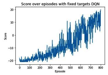
From the preceding image, we can see that the agent gradually learned to play Pong and that by the end of 800 episodes, it learned how to play Pong while receiving a high reward.
Now that we've trained an agent to play Pong well, in the next section, we will train an agent so that it can drive a car autonomously in a simulated environment.
Implementing an agent to perform autonomous driving
Now that you have seen RL working in progressively challenging environments, we will conclude this chapter by demonstrating that the same concepts can be applied to a self-driving car. Since it is impractical to see this working on an actual car, we will resort to a simulated environment. The environment is going to be a full-fledged city of traffic, with cars and additional details within the image of a road. The actor (agent) is a car. The inputs to the car are going to be various sensory inputs such as a dashcam, Light Detection And Ranging (LIDAR) sensors, and GPS coordinates. The outputs are going to be how fast/slow the car will move, along with the level of steering. This simulation will attempt to be an accurate representation of real-world physics. Thus, note that the fundamentals will remain the same, whether it is a car simulation or a real car.
Installing the CARLA environment
As we mentioned previously, we need an environment that can simulate complex interactions to make us believe that we are, in fact, dealing with a realistic scenario. CARLA is one such environment. The environment author stated the following about CARLA:
There are two steps we need to follow to install the environment:
- Install the CARLA binaries for the simulation environment.
- Install the Gym version, which provides Python connectivity for the simulation environment.
Let's get started!
Install the CARLA binaries
In this section, we will learn how to install the necessary CARLA binaries:
- Visit https://github.com/carla-simulator/carla/releases/tag/0.9.6 and download the CARLA_0.9.6.tar.gz compiled version file.
- Move it to a location where you want CARLA to live in your system and unzip it. Here, we are demonstrating this by downloading and unzipping CARLA into the Documents folder:
$ mv CARLA_0.9.6.tar.gz ~/Documents/
$ cd ~/Documents/
$ tar -xf CARLA_0.9.6.tar.gz
$ cd CARLA_0.9.6/
- Add CARLA to PYTHONPATH so that any module on your machine can import CARLA:
$ echo "export PYTHONPATH=$PYTHONPATH:/home/$(whoami)/Documents/CARLA_0.9.6/PythonAPI/carla/dist/carla-0.9.6-py3.5-linux-x86_64.egg" >> ~/.bashrc
In the preceding code, we added the directory containing CARLA to a global variable called PYTHONPATH, which is an environment variable for accessing all Python modules. Adding it to ~/.bashrc will ensure that every time a Terminal is opened, it can access this new folder. After running the preceding code, restart the Terminal and run ipython -c "import carla; carla.__spec__". You should get the following output:

- Finally, provide the necessary permissions and execute CARLA, as follows:
$ chmod +x /home/$(whoami)/Documents/CARLA_0.9.6/CarlaUE4.sh
$ ./home/$(whoami)/Documents/CARLA_0.9.6/CarlaUE4.sh
After a minute or two, you should see a window similar to the following showing CARLA running as a simulation, ready to take inputs:

In this section, we've verified that CARLA is a simulation environment whose binaries are working as expected. Let's move on to installing the Gym environment for it. Leave the Terminal running as-is since we need the binary to be running in the background throughout this exercise.
Installing the CARLA Gym environment
Since there is no official Gym environment, we will take advantage of a user implemented GitHub repository and install the Gym environment for CARLA from there. Follow these steps to install CARLA's Gym environment:
- Clone the Gym repository to a location of your choice and install the library:
$ cd /location/to/clone/repo/to
$ git clone https://github.com/cjy1992/gym-carla
$ cd gym-carla
$ pip install -r requirements.txt
$ pip install -e .
- Test your setup by running the following command:
$ python test.py
A window similar to the following should open, showing that we have added a fake car to the environment. From here, we can monitor the top view, the LIDAR sensor point cloud, and our dashcam:

Here, we can observe the following:
- The first view contains a view that is very similar to what vehicle GPS systems show in a car; that is, our vehicle, the various waypoints, and the road lanes. However, we shall not use this input for training as it also shows other cars in the view, which is unrealistic.
- The second view is more interesting. Some consider it as the eye of a self-driving car. LIDAR emits pulsed light into the surrounding environment (in all directions), multiple times every second. It captures the reflected light to determine how far the nearest obstacle is in that direction. The onboard computer collates all the nearest obstacle information to recreate a 3D point cloud that gives it a 3D understanding of its environment.
- In both the first and second views, we can see there is a strip ahead of the car. This is a waypoint indication of where the car is supposed to go.
- The third view is a simple dashboard camera.
Apart from these three, CARLA provides additional sensor data, such as the following:
- lateral-distance (deviation from the lane it should be in)
- delta-yaw (angle with respect to the road ahead)
- speed
- If there's a hazardous obstacle in front of the vehicle
- And many more...
We are going to use the first four sensors mentioned previously, along with LIDAR and our dashcam, to train the model.
We are now ready to understand the components of CARLA and create a DQN model for a self-driving car.
Training a self-driving agent
We will create two files before we start the training process in a notebook; that is, model.py and actor.py. These will contain the model architecture and the Agent class, respectively. The Agent class contains the various methods we'll use to train an agent.
model.py
This is going to be a PyTorch model that will accept the image that's provided to it, as well as other sensor inputs. It will be expected to return the most likely action:
from torch_snippets import *

class DQNetworkImageSensor(nn.Module):
    def __init__(self):
        super().__init__()
        self.n_outputs = 9
        self.image_branch = nn.Sequential(
                            nn.Conv2d(3, 32, (8, 8), stride=4),
                            nn.ReLU(inplace=True),
                            nn.Conv2d(32, 64, (4, 4), stride=2),
                            nn.ReLU(inplace=True),
                            nn.Conv2d(64,128,(3, 3),stride=1),
                            nn.ReLU(inplace=True),
                            nn.AvgPool2d(8),
                            nn.ReLU(inplace=True),
                            nn.Flatten(),
                            nn.Linear(1152, 512),
                            nn.ReLU(inplace=True),
                            nn.Linear(512, self.n_outputs)
                        )

        self.lidar_branch = nn.Sequential(
                            nn.Conv2d(3, 32, (8, 8), stride=4),
                            nn.ReLU(inplace=True),
                            nn.Conv2d(32,64,(4, 4),stride=2),
                            nn.ReLU(inplace=True),
                            nn.Conv2d(64,128,(3, 3),stride=1),
                            nn.ReLU(inplace=True),
                            nn.AvgPool2d(8),
                            nn.ReLU(inplace=True),
                            nn.Flatten(),
                            nn.Linear(1152, 512),
                            nn.ReLU(inplace=True),
                            nn.Linear(512, self.n_outputs)
                        )

        self.sensor_branch = nn.Sequential(
                                nn.Linear(4, 64),
                                nn.ReLU(inplace=True),
                                nn.Linear(64, self.n_outputs)
                            )

    def forward(self, image, lidar=None, sensor=None):
        x = self.image_branch(image)
        if lidar is None:
            y = 0
        else:
            y = self.lidar_branch(lidar)
        z = self.sensor_branch(sensor)

        return x + y + z
As you can see, there are more types of data being fed into the forward method than in the previous sections, where we were just accepting an image as input. self.image_branch is going to expect the image coming from the dashcam of the car, while self.lidar_branch will accept the image that's generated by the LIDAR sensor. Finally, self.sensor_branch will accept four sensor inputs in the form of a NumPy array. These four items are the lateral-distance (deviation from the lane it is supposed to be in), delta-yaw (angle with respect to the road ahead), speed, and if there's a hazardous obstacle at the front of the vehicle, respectively. See line number 543 in gym_carla/envs/carla_env.py (the repository that has been git cloned) for the same outputs. Using a different branch in the neural network will let the module provide different levels of importance for each sensor, and the outputs are summed up as the final output. Note that there are 9 outputs; we will look at these later.
actor.py
Much like the previous sections, we will use some code to store replay information and play it back when training is necessary:
- Let's get the imports and hyperparameters in place:
import numpy as np
import random
from collections import namedtuple, deque
import torch
import torch.nn.functional as F
import torch.optim as optim
from model1 import DQNetworkImageSensor

BUFFER_SIZE = int(1e3) # replay buffer size
BATCH_SIZE = 256 # minibatch size
GAMMA = 0.99 # discount factor
TAU = 1e-2 # for soft update of target parameters
LR = 5e-4 # learning rate
UPDATE_EVERY = 50 # how often to update the network
ACTION_SIZE = 2

device = 'cuda' if torch.cuda.is_available() else 'cpu'
- Next, we'll initialize the target and local networks. No changes have been made to the code from the previous section here, except for the module that is being imported:
class Actor():
    def __init__(self):
        # Q-Network
        self.qnetwork_local=DQNetworkImageSensor().to(device)
        self.qnetwork_target=DQNetworkImageSensor().to(device)
        self.optimizer = optim.Adam(self.qnetwork_local
                                    .parameters(),lr=LR)

        # Replay memory
        self.memory= ReplayBuffer(ACTION_SIZE,BUFFER_SIZE,
                                   BATCH_SIZE, 10)
        # Initialize time step
        # (for updating every UPDATE_EVERY steps)
        self.t_step = 0

    def step(self, state, action, reward, next_state, done):
        # Save experience in replay memory
        self.memory.add(state, action, reward,
                        next_state, done)

        # Learn every UPDATE_EVERY time steps.
        self.t_step = (self.t_step + 1) % UPDATE_EVERY
        if self.t_step == 0:
  # If enough samples are available in memory,
  # get random subset and learn
            if len(self.memory) > BATCH_SIZE:
                experiences = self.memory.sample()
                self.learn(experiences, GAMMA)
- Since there are more sensors to handle, we'll transport them as a dictionary of state. The state contains the 'image', 'lidar', and 'sensor' keys, which we introduced in the previous section. We perform preprocessing before sending them to the neural network, as shown in the following code:
    def act(self, state, eps=0.):
        images,lidars sensors=state['image'],
                              state['lidar'],state['sensor']
        images = torch.from_numpy(images).float()
                      .unsqueeze(0).to(device)
        lidars = torch.from_numpy(lidars).float()
                      .unsqueeze(0).to(device)
        sensors = torch.from_numpy(sensors).float()
                       .unsqueeze(0).to(device)
        self.qnetwork_local.eval()
        with torch.no_grad():
            action_values = self.qnetwork_local(images,
                                lidar=lidars, sensor=sensors)
        self.qnetwork_local.train()
        # Epsilon-greedy action selection
        if random.random() > eps:
            return np.argmax(action_values.cpu().data.numpy())
        else:
            return random.choice(np.arange(
                        self.qnetwork_local.n_outputs))
- Now, we need to fetch items from replay memory. The following instructions are being executed in the following code:
- Obtain a batch of current and next states.
- Compute the expected reward, Q_expected, if a network performs actions in the current state.
- Compare it with the target reward, Q_targets, that would have been obtained when the next state was fed to the network.
- Periodically update the target network with the local network:
    def learn(self, experiences, gamma):
        states,actions,rewards,next_states,dones= experiences
        images, lidars, sensors = states
        next_images, next_lidars, next_sensors = next_states
        # Get max predicted Q values (for next states)
        # from target model
        Q_targets_next = self.qnetwork_target(next_images,
                       lidar=next_lidars,sensor=next_sensors)
                            .detach().max(1)[0].unsqueeze(1)
        # Compute Q targets for current states
        Q_targets = rewards +(gamma*Q_targets_next*(1-dones))

        # Get expected Q values from local model
        # import pdb; pdb.set_trace()
        Q_expected=self.qnetwork_local(images,lidar=lidars,
                   sensor=sensors).gather(1,actions.long())
        # Compute loss
        loss = F.mse_loss(Q_expected, Q_targets)
        # Minimize the loss
        self.optimizer.zero_grad()
        loss.backward()
        self.optimizer.step()

        # ------------ update target network ------------- #
        self.soft_update(self.qnetwork_local,
                         self.qnetwork_target, TAU)

    def soft_update(self, local_model, target_model, tau):
        for target_param, local_param in
            zip(target_model.parameters(),
            local_model.parameters()):
            target_param.data.copy_(tau*local_param.data +
                                (1.0-tau)*target_param.data)
- The only major change in the ReplayBuffer class is going to be how the data is stored. Since we have multiple sensors, each memory (states and next_states) is stored as a tuple of data; that is, states = [images, lidars, sensors]:
class ReplayBuffer:
    """Fixed-size buffer to store experience tuples."""
    def __init__(self, action_size, buffer_size,
                 batch_size, seed):
        self.action_size = action_size
        self.memory = deque(maxlen=buffer_size)
        self.batch_size = batch_size
        self.experience = namedtuple("Experience",
                          field_names=["state", "action",
                                     "reward","next_state",
                                       "done"])
        self.seed = random.seed(seed)

    def add(self, state, action, reward, next_state, done):
        """Add a new experience to memory."""
        e = self.experience(state, action, reward,
                            next_state, done)
        self.memory.append(e)


    def sample(self):
        experiences = random.sample(self.memory,
                                    k=self.batch_size)
        images = torch.from_numpy(np.vstack(
                    [e.state['image'][None]
                 for e in experiences if e is not None]))
                    .float().to(device)
        lidars = torch.from_numpy(np.vstack(
                    [e.state['lidar'][None]
                 for e in experiences if e is not None]))
                    .float().to(device)
        sensors = torch.from_numpy(np.vstack(
                    [e.state['sensor']
                 for e in experiences if e is not None]))
                    .float().to(device)
        states = [images, lidars, sensors]
        actions = torch.from_numpy(np.vstack(
                    [e.action for e in experiences
                     if e is not None])).long().to(device)
        rewards = torch.from_numpy(np.vstack(
                    [e.reward for e in experiences
                     if e is not None])).float().to(device)
        next_images = torch.from_numpy(np.vstack(
                    [e.next_state['image'][None]
                     for e in experiences if e is not None]))
                    .float().to(device)
        next_lidars = torch.from_numpy(np.vstack(
                    [e.next_state['lidar'][None]
                     for e in experiences if e is not None]))
                    .float().to(device)
        next_sensors = torch.from_numpy(np.vstack(
                    [e.next_state['sensor']
                     for e in experiences if e is not None]))
                    .float().to(device)
        next_states = [next_images, next_lidars, next_sensors]
        dones = torch.from_numpy(np.vstack([e.done
                     for e in experiences if e is not None])
                    .astype(np.uint8)).float().to(device)

        return (states, actions, rewards, next_states, dones)

    def __len__(self):
        """Return the current size of internal memory."""
        return len(self.memory)
Note that the lines of code in bold fetch the current states, actions, rewards, and next states' information.
Now that the critical components are in place, let's load the Gym environment into a Python notebook and start training.
Training DQN with fixed targets
There is no additional theory we need to learn here. The basics remain the same; we'll only be making changes to the Gym environment, the architecture of the neural network, and the actions our agent needs to take:
- First, load the hyperparameters associated with the environment. Refer to each comment beside every key-value pair presented in the params dictionary in the following code. Since we are simulating a complex environment, we need to choose the environment's parameters, such as the number of cars in the city, number of walkers, which town to simulate, the resolution of the dashcam image, and LIDAR sensors:
import gym
import gym_carla
import carla
from model import DQNetworkState
from actor import Actor
from torch_snippets import *

params = {
    'number_of_vehicles': 10,
    'number_of_walkers': 0,
    'display_size': 256, # screen size of bird-eye render
    'max_past_step': 1, # the number of past steps to draw
    'dt': 0.1, # time interval between two frames
    'discrete': True, # whether to use discrete control space
    # discrete value of accelerations
    'discrete_acc': [-1, 0, 1],
    # discrete value of steering angles
    'discrete_steer': [-0.3, 0.0, 0.3],
    # define the vehicle
    'ego_vehicle_filter': 'vehicle.lincoln*',
    'port': 2000, # connection port
    'town': 'Town03', # which town to simulate
    'task_mode': 'random', # mode of the task
    'max_time_episode': 1000, # maximum timesteps per episode
    'max_waypt': 12, # maximum number of waypoints
    'obs_range': 32, # observation range (meter)
    'lidar_bin': 0.125, # bin size of lidar sensor (meter)
    'd_behind': 12, # distance behind the ego vehicle (meter)
    'out_lane_thres': 2.0, # threshold for out of lane
    'desired_speed': 8, # desired speed (m/s)
    'max_ego_spawn_times': 200, # max times to spawn vehicle
    'display_route': True, # whether to render desired route
    'pixor_size': 64, # size of the pixor labels
    'pixor': False, # whether to output PIXOR observation
}

# Set gym-carla environment
env = gym.make('carla-v0', params=params)
In the preceding params dictionary, the following are important for our simulation in terms of the action space:
- 'discrete': True: Our actions lie in a discrete space.
- 'discrete_acc':[-1,0,1]: All the possible accelerations the self-driven car is allowed to make during the simulation.
- 'discrete_steer':[-0.3,0,0.3]: All the possible steering magnitudes, the self-driven car is allowed to make during the simulation.
Feel free to change the parameters once you've gone through the official documentation.
- With that, we have all the components we need to train the model. Load a pre-trained model, if one exists:
load_path = None # 'car-v1.pth'
# continue training from an existing model
save_path = 'car-v2.pth'

actor = Actor()
if load_path is not None:
    actor.qnetwork_local.load_state_dict(
                            torch.load(load_path))
    actor.qnetwork_target.load_state_dict(
                            torch.load(load_path))
else:
    pass
- Fix the number of episodes and define the dqn function to train the agent, as follows:
- Reset the state:
n_episodes = 100000
def dqn(n_episodes=n_episodes, max_t=1000, eps_start=1,
        eps_end=0.01, eps_decay=0.995):
    scores = [] # list containing scores from each episode
    scores_window = deque(maxlen=100) # last 100 scores
    eps = eps_start # Initialize epsilon
    for i_episode in range(1, n_episodes+1):
        state = env.reset()
- Wrap the state into a dictionary (as discussed in the actor.py:Actor class) and act on it:
        image, lidar, sensor = state['camera'],
                               state['lidar'],
                               state['state']
        image, lidar = preprocess(image), preprocess(lidar)
        state_dict = {'image': image, 'lidar': lidar,
                      'sensor': sensor}
        score = 0
        for t in range(max_t):
            action = actor.act(state_dict, eps)
- Store the next state that's obtained from the environment and then store the state, next_state pair (along with the rewards and other state information) to train the actor using DQN:
            next_state, reward, done, _ = env.step(action)
            image, lidar, sensor = next_state['camera'],
                                   next_state['lidar'],
                                   next_state['state']
            image,lidar = preprocess(image), preprocess(lidar)
            next_state_dict = {'image':image,'lidar':lidar,
                               'sensor': sensor}
            actor.step(state_dict, action, reward,
                       next_state_dict, done)
            state_dict = next_state_dict
            score += reward
            if done:
                break
        scores_window.append(score) # save most recent score
        scores.append(score) # save most recent score
        eps = max(eps_end, eps_decay*eps) # decrease epsilon
        if i_episode % 100 == 0:
            log.record(i_episode,
                       mean_score=np.mean(scores_window))
            torch.save(actor.qnetwork_local.state_dict(),
                       save_path)
We must repeat the loop until we get a done signal, after which we reset the environment and start storing actions once again. After every 100 episodes, store the model.
- Call the dqn function to train the model:
dqn()
Since this is a more complex environment, training can take a few days, so be patient and continue training a few hours at a time using the load_path and save_path arguments. With enough training, the vehicle can maneuver and learn how to drive by itself. Here's a video of the training result we were able to achieve after two days of training: https://tinyurl.com/mcvp-self-driving-agent-result.
Summary
In this chapter, we learned how the values of various actions in a given state are calculated. We then learned how the agent updates the Q-table using the discounted value of taking an action in a given state. In the process of doing this, we learned how the Q-table is infeasible in a scenario where the number of states is high. We also learned how to leverage deep Q-networks to address the scenario where the number of possible states is high. Next, we moved on to leveraging CNN-based neural networks while building an agent that learned how to play Pong using DQN based on fixed targets. Finally, we learned how to leverage DQN with fixed targets to perform self-driving using the CARLA simulator. As we have seen repeatedly in this chapter, you can use deep Q-learning to learn very different tasks – such as CartPole balancing, playing Pong, and self-driving navigation – with almost the same code. While this is not the end of our journey into exploring RL, at this point, we should be able to appreciate how we can use CNN-based and reinforcement learning-based algorithms together to solve complex problems and build learning agents.
So far, we have learned how to combine computer vision-based techniques with techniques from other prominent areas of research, including meta-learning, natural language processing, and reinforcement learning. Apart from this, we've also learned how to perform object classification, detection, segmentation, and image generation using GANs. In the next chapter, we will switch gears and learn how to move a deep learning model to production.
Questions
- How is a value calculated for a given state?
- How is a Q-table populated?
- Why do we have a discount factor in the state-action value calculation?
- What do we need the exploration-exploitation strategy?
- Why do we need to use deep Q-learning?
- How is the value of a given state-action combination calculated using deep Q-learning?
- Once the agent has maximized the reward in the CartPole environment, is there a chance that it can learn a sub-optimal policy later?