So far, in the previous chapters, we learned about performing image classification. Imagine a scenario where we are leveraging computer vision for a self-driving car. It is not only necessary to detect whether the image of a road contains the images of vehicles, a sidewalk, and pedestrians, but it is also important to identify where those objects are located. Various techniques of object detection that we will study in this chapter and the next will come in handy in such a scenario.

In this chapter and the next, we will learn about some of the techniques for performing object detection. We will start by learning about the fundamentals—labeling the ground truth of bounding box objects using a tool named ybat, extracting region proposals using the selectivesearch method, and defining the accuracy of bounding box predictions by using the Intersection over Union (IoU) metric and the mean average precision metric. After this, we will learn about two region proposal-based networks – R-CNN and Fast R-CNN, by first learning about their working details and then implementing them on a dataset that contains images belonging to trucks and buses.

The following topics will be covered in this chapter:

• Introducing object detection
• Creating a bounding box ground truth for training
• Understanding region proposals
• Understanding IoU, non-max suppression, and mean average precision
• Training R-CNN-based custom object detectors
• Training Fast R-CNN-based custom object detectors

Introducing object detection

With the rise of autonomous cars, facial detection, smart video surveillance, and people-counting solutions, fast and accurate object detection systems are in great demand. These systems include not only object classification from an image, but also location of each one of the objects by drawing appropriate bounding boxes around them. This (drawing bounding boxes and classification) makes object detection a harder task than its traditional computer vision predecessor, image classification.

To understand what the output of object detection looks like, let's go through the following diagram:

In the preceding diagram, we can see that, while a typical object classification merely mentions the class of object present in the image, object localization draws a bounding box around the objects present in the image. Object detection, on the other hand, would involve drawing the bounding boxes around individual objects in the image, along with identifying the class of object within a bounding box across the multiple objects present in the image.

Before we understand the broad use cases of object detection, let's understand how it adds to the object classification task that we have covered in the previous chapter.

Imagine a scenario where you have multiple objects in an image. I ask you to predict the class of objects present in the image. For example, let's say that the image contains both cats and dogs. How would you classify such images? Object detection comes in handy in such a scenario, where it not only predicts the location of objects (bounding box) present in it, but also predicts the class of object present within the individual bounding boxes.

Some of the various use cases leveraging object detection include the following:

• Security: This can be useful for recognizing intruders.
• Autonomous cars: This can be helpful in recognizing the various objects present on the image of a road.
• Image searching: This can help identify the images containing an object (or a person) of interest.
• Automotives: This can help in identifying a number plate within the image of a car.

In all the preceding cases, object detection is leveraged to draw bounding boxes around a variety of objects present within the image.

In this chapter, we will learn about predicting the class of the object and also having a tight bounding box around the object in the image, which is the localization task. We will also learn about detecting the class corresponding to multiple objects in the picture, along with a bounding box around each object, which is the object detection task.

Training a typical object detection model involves the following steps:

1. Creating ground truth data that contains labels of the bounding box and class corresponding to various objects present in the image.
2. Coming up with mechanisms that scan through the image to identify regions (region proposals) that are likely to contain objects. In this chapter, we will learn about leveraging region proposals generated by a method named selective search. In the next chapter, we will learn about leveraging anchor boxes to identify regions containing objects. In the chapter on combining computer vision and NLP techniques (Chapter 15), we will learn about leveraging positional embeddings in transformers to aid in identifying the regions containing an object.
3. Creating the target class variable by using the IoU metric.
4. Creating the target bounding box offset variable to make corrections to the location of region proposal coming in the second step.
5. Building a model that can predict the class of object along with the target bounding box offset corresponding to the region proposal.
6. Measuring the accuracy of object detection using mean Average Precision (mAP).

Now that we have a high-level overview of what is to be done to train an object detection model, we will learn about creating the dataset for a bounding box (which is the first step in building an object detection model) in the next section.

Creating a bounding box ground truth for training

We have learned that object detection gives us the output where a bounding box surrounds the object of interest in an image. For us to build an algorithm that detects the bounding box surrounding the object in an image, we would have to create the input-output combinations, where the input is the image and the output is the bounding boxes surrounding the objects in the given image, and the classes corresponding to the objects.

To train a model that provides the bounding box, we need the image, and also the corresponding bounding box coordinates of all the objects in an image. In this section, we will learn about one way to create the training dataset, where the image is the input and the corresponding bounding boxes and classes of objects are stored in an XML file as output. We will use the ybat tool to annotate the bounding boxes and the corresponding classes.

Let's understand about installing and using ybat to create (annotate) bounding boxes around objects in the image. Furthermore, we will also be inspecting the XML files that contain the annotated class and bounding box information in the following section.

Installing the image annotation tool

Let's start by downloading ybat-master.zip from the following GitHub link, https://github.com/drainingsun/ybat, and unzip it. Post unzipping, store it in a folder of your choice. Open ybat.html using a browser of your choice and you will see an empty page. The following screenshot shows a sample of what the folder looks like and how to open the ybat.html file:

Before we start creating the ground truth corresponding to an image, let's specify all the possible classes that we want to label across images and store in the classes.txt file as follows:

Now, let's prepare the ground truth corresponding to an image. This involves drawing a bounding box around objects (persons in the following diagram) and assigning labels/classes to the objects present in the image in the following steps:

1. Upload all the images you want to annotate (step number 1 in the following image).
2. Upload the classes.txt file (step number 2 in the following image).
3. Label each image by first selecting the filename and then drawing a crosshair around each object you want to label (step number 3 in the following image). Before drawing a crosshair, ensure you select the correct class in the classes region (the classes pane below the second oval in the following image).
4. Save the data dump in the desired format (step number 4 in the following image). Each format was independently developed by a different research team, and all are equally valid. Based on their popularity and convenience, every implementation prefers a different format.

All these steps can be better represented using the following diagram:

For example, when we download the PascalVOC format, it downloads a zip of XML files. A snapshot of the XML file after drawing the rectangular bounding box is as follows:

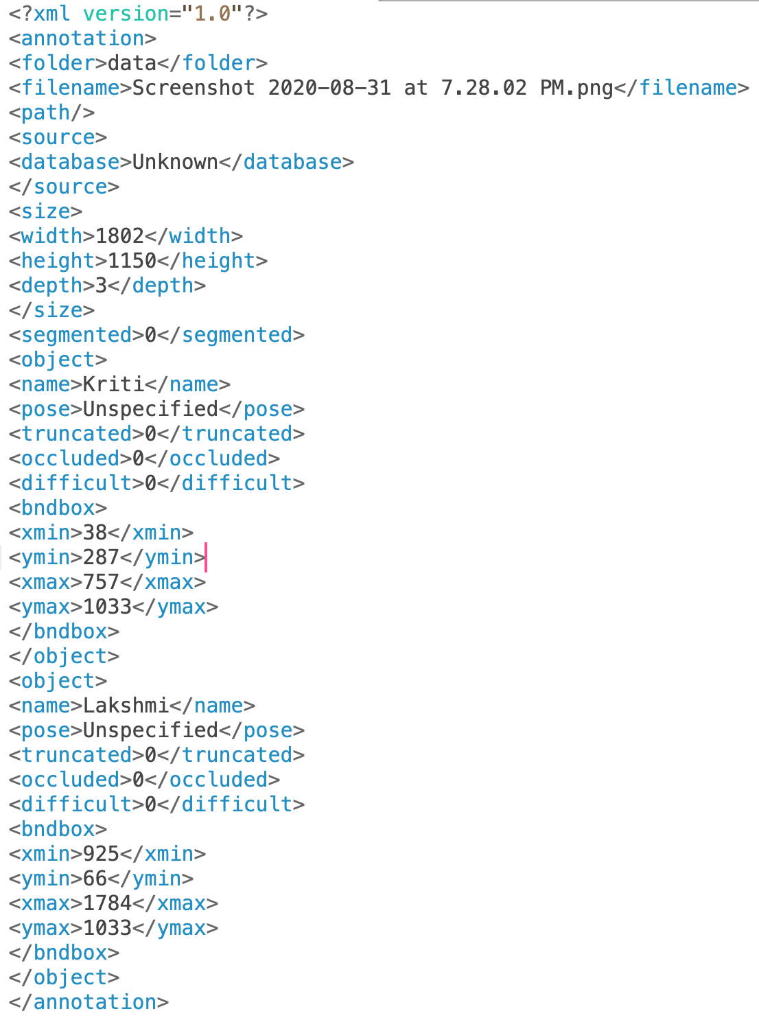
From the preceding screenshot, note that the bndbox field contains the coordinates of the minimum and maximum values of the x and y coordinates corresponding to the objects of interest in the image. We should also be able to extract the classes corresponding to the objects in the image using the name field.

Now that we understand how to create a ground truth of objects (class label and bounding box) present in an image, in the following sections, we will dive into the building blocks of recognizing objects in an image. First, we will talk about region proposals that help in highlighting the portions of the image that are most likely to contain an object.

Understanding region proposals

Imagine a hypothetical scenario where the image of interest contains a person and sky in the background. Furthermore, for this scenario, let's assume that there is little change in pixel intensity of the background (sky) and that there is a considerable change in pixel intensity of the foreground (the person).

Just from the preceding description itself, we can conclude that there are two primary regions here – one is of the person and the other is of the sky. Furthermore, within the region of the image of a person, the pixels corresponding to hair will have a different intensity to the pixels corresponding to the face, establishing that there can be multiple sub-regions within a region.

Region proposal is a technique that helps in identifying islands of regions where the pixels are similar to one another.

Generating a region proposal comes in handy for object detection where we have to identify the locations of objects present in the image. Furthermore, given a region proposal generates a proposal for the region, it aids in object localization where the task is to identify a bounding box that fits exactly around the object in the image. We will learn how region proposals assist in object localization and detection in a later section on Training R-CNN-based custom object detectors, but let's first understand how to generate region proposals from an image.

Leveraging SelectiveSearch to generate region proposals

SelectiveSearch is a region proposal algorithm used for object localization where it generates proposals of regions that are likely to be grouped together based on their pixel intensities. SelectiveSearch groups pixels based on the hierarchical grouping of similar pixels, which, in turn, leverages the color, texture, size, and shape compatibility of content within an image.

Initially, SelectiveSearch over-segments an image by grouping pixels based on the preceding attributes. Next, it iterates through these over-segmented groups and groups them based on similarity. At each iteration, it combines smaller regions to form a larger region.

Let's understand the selectivesearch process through the following example:

1. Install the required packages:

!pip install selectivesearch
!pip install torch_snippets
from torch_snippets import *
import selectivesearch
from skimage.segmentation import felzenszwalb

2. Fetch and load the required image:

!wget https://www.dropbox.com/s/l98leemr7r5stnm/Hemanvi.jpeg
img = read('Hemanvi.jpeg', 1)

3. Extract the felzenszwalb segments (which are obtained based on the color, texture, size, and shape compatibility of content within an image) from the image:

segments_fz = felzenszwalb(img, scale=200)

Note that in the felzenszwalb method, scale represents the number of clusters that can be formed within the segments of the image. The higher the value of scale, the greater the detail of the original image that is preserved.

4. Plot the original image and the image with segmentation:

subplots([img, segments_fz], 
         titles=['Original Image',
                 'Image post
felzenszwalb segmentation'],
         sz=10, nc=2)

The preceding code results in the following output:

From the preceding output, note that pixels that belong to the same group have similar pixel values.

Now that we understand what SelectiveSearch does, let's implement the selectivesearch function to fetch region proposals for the given image.

Implementing SelectiveSearch to generate region proposals

In this section, we will define the extract_candidates function using selectivesearch so that it can be leveraged in the subsequent sections on training R-CNN- and Fast R-CNN-based custom object detectors:

1. Define the extract_candidates function that fetches the region proposals from an image:

• Define the function that takes an image as the input parameter:

def extract_candidates(img):

• Fetch the candidate regions within the image using the selective_search method available in the selectivesearch package:

    img_lbl, regions = selectivesearch.selective_search(img, 
                                     scale=200, min_size=100)

• Calculate the image area and initialize a list (candidates) that we will use to store the candidates that pass a defined threshold:

    img_area = np.prod(img.shape[:2])
    candidates = []

• Fetch only those candidates (regions) that are over 5% of the total image area and less than or equal to 100% of the image area and return them:

    for r in regions:
        if r['rect'] in candidates: continue
        if r['size'] < (0.05*img_area): continue
        if r['size'] > (1*img_area): continue
        x, y, w, h = r['rect']
        candidates.append(list(r['rect']))
    return candidates

2. Import the relevant packages and fetch an image:

!pip install selectivesearch
!pip install torch_snippets
from torch_snippets import *
import selectivesearch
!wget https://www.dropbox.com/s/l98leemr7r5stnm/Hemanvi.jpeg
img = read('Hemanvi.jpeg', 1)

3. Extract candidates and plot them on top of an image:

candidates = extract_candidates(img)
show(img, bbs=candidates)

The preceding code generates the following output:

The grids in the preceding diagram represent the candidate regions (region proposals) coming from the selective_search method.

Now that we understand region proposal generation, one question remains unanswered. How do we leverage region proposals for object detection and localization?

A region proposal that has a high intersection with the location (ground truth) of an object in the image of interest is labeled as the one that contains the object, and a region proposal with a low intersection is labeled as background.

In the next section, we will learn about how to calculate the intersection of a region proposal candidate with a ground truth bounding box in our journey to understanding the various techniques that form the backbone of building an object detection model.

Understanding IoU

Imagine a scenario where we came up with a prediction of a bounding box for an object. How do we measure the accuracy of our prediction? The concept of Intersection over Union (IoU) comes in handy in such a scenario.

Intersection within the term Intersection over Union measures how overlapping the predicted and actual bounding boxes are, while Union measures the overall space possible for overlap. IoU is the ratio of the overlapping region between the two bounding boxes over the combined region of both the bounding boxes.

This can be represented in a diagram as follows:

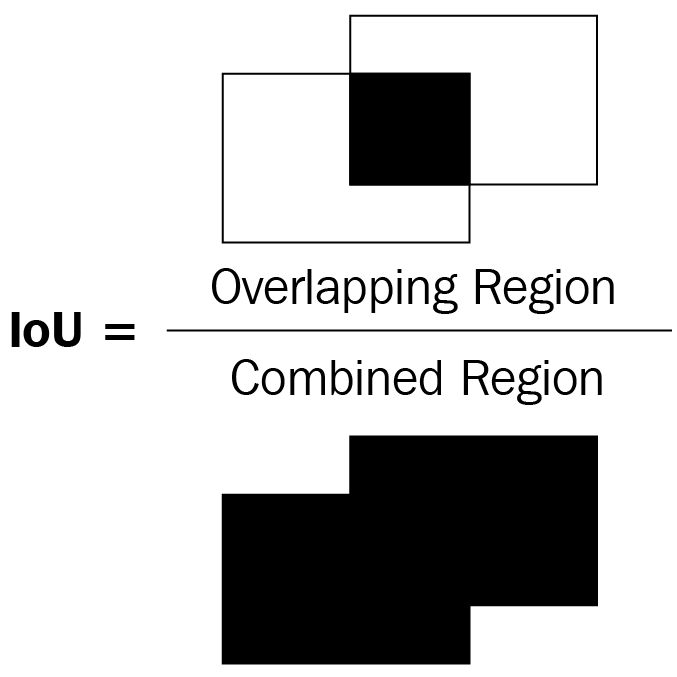
In the preceding diagram of two bounding boxes (rectangles), let's consider the left bounding box as the ground truth and the right bounding box as the predicted location of the object. IoU as a metric is the ratio of the overlapping region over the combined region between the two bounding boxes.

In the following diagram, you can observe the variation in the IoU metric as the overlap between bounding boxes varies:

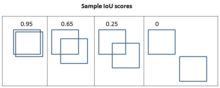
From the preceding diagram, we can see that as the overlap decreases, IoU decreases and, in the final one, where there is no overlap, the IoU metric is 0.

Now that we have an intuition of measuring IoU, let's implement it in code and create a function to calculate IoU as we will leverage it in the sections of training R-CNN and training Fast R-CNN.

Let's define a function that takes two bounding boxes as input and returns IoU as the output:

1. Specify the get_iou function that takes boxA and boxB as inputs where boxA and boxB are two different bounding boxes (you can consider boxA as the ground truth bounding box and boxB as the region proposal):

def get_iou(boxA, boxB, epsilon=1e-5):

We define the epsilon parameter to address the rare scenario when the union between the two boxes is 0, resulting in a division by zero error. Note that in each of the bounding boxes, there will be four values corresponding to the four corners of the bounding box.

2. Calculate the coordinates of the intersection box:

    x1 = max(boxA[0], boxB[0])
    y1 = max(boxA[1], boxB[1])
    x2 = min(boxA[2], boxB[2])
    y2 = min(boxA[3], boxB[3])

Note that x1 is storing the maximum value of the left-most x-value between the two bounding boxes. Similarly, y1 is storing the topmost y-value and x2 and y2 are storing the right-most x-value and bottom-most y-value, respectively, corresponding to the intersection part.

3. Calculatewidth and height corresponding to the intersection area (overlapping region):

    width = (x2 - x1)
    height = (y2 - y1)

4. Calculate the area of overlap (area_overlap):

    if (width<0) or (height <0):
        return 0.0
    area_overlap = width * height

Note that, in the preceding code, we specify that if the width or height corresponding to the overlapping region is less than 0, the area of intersection is 0. Otherwise, we calculate the area of overlap (intersection) similar to the way a rectangle's area is calculated – width multiplied by the height.

5. Calculate the combined area corresponding to the two bounding boxes:

    area_a = (boxA[2] - boxA[0]) * (boxA[3] - boxA[1])
    area_b = (boxB[2] - boxB[0]) * (boxB[3] - boxB[1])
    area_combined = area_a + area_b - area_overlap

In the preceding code, we have calculated the combined area of the two bounding boxes – area_a and area_b, and then subtracted the overlapping area while calculating area_combined as area_overlap is counted twice, once when calculating area_a and then when calculating area_b.

6. Calculate the IoU and return it:

    iou = area_overlap / (area_combined+epsilon)
    return iou

In the preceding code, we calculated iou as the ratio of the area of overlap (area_overlap) over the area of the combined region (area_combined) and returning it.

So far, we have learned about creating ground truth and calculating IoU, which helps in preparing training data. Next, the object detection models will come in handy in detecting objects in the image. Finally, we will calculate model performance and infer on a new image.

We will hold off on building a model until the forthcoming sections as training a model is more involved and we would also have to learn a few more components before we train it. In the next section, we will learn about non-max suppression, which helps in shortlisting from the different possible predicted bounding boxes around an object when inferring using the trained model on a new image.

Non-max suppression

Imagine a scenario where multiple region proposals are generated and significantly overlap one another. Essentially, all the predicted bounding box coordinates (offsets to region proposals) significantly overlap one another. For example, let's consider the following image, where multiple region proposals are generated for the person in the image:

In the preceding image, I ask you to identify the box among the many region proposals that we will consider as the one containing an object and the boxes that we will discard. Non-max suppression comes in handy in such a scenario. Let's unpack the term "Non-max suppression."

Non-max refers to the boxes that do not contain the highest probability of containing an object, and suppression refers to us discarding those boxes that do not contain the highest probabilities of containing an object. In non-max suppression, we identify the bounding box that has the highest probability and discard all the other bounding boxes that have an IoU greater than a certain threshold with the box containing the highest probability of containing an object.

In PyTorch, non-max suppression is performed using the nms function in the torchvision.ops module. The nms function takes the bounding box coordinates, the confidence of the object in the bounding box, and the threshold of IoU across bounding boxes, to identify the bounding boxes to be retained. You will be leveraging the nms function when predicting object classes and bounding boxes of objects in a new image in both the Training R-CNN-based custom object detectors and Training Fast R-CNN-based custom object detectors sections in steps 19 and 16, respectively.

Mean average precision

So far, we have looked at getting an output that comprises a bounding box around each object within the image and the class corresponding to the object within the bounding box. Now comes the next question: How do we quantify the accuracy of the predictions coming from our model?

mAP comes to the rescue in such a scenario. Before we try to understand mAP, let's first understand precision, then average precision, and finally, mAP:

• Precision: Typically, we calculate precision as:

A true positive refers to the bounding boxes that predicted the correct class of objects and that have an IoU with the ground truth that is greater than a certain threshold. A false positive refers to the bounding boxes that predicted the class incorrectly or have an overlap that is less than the defined threshold with the ground truth. Furthermore, if there are multiple bounding boxes that are identified for the same ground truth bounding box, only one box can get into a true positive, and everything else gets into a false positive.

• Average Precision: Average precision is the average of precision values calculated at various IoU thresholds.
• mAP: mAP is the average of precision values calculated at various IoU threshold values across all the classes of objects present within the dataset.

So far, we have learned about preparing a training dataset for our model, performing non-max suppression on the model's predictions, and calculating its accuracies. In the following sections, we will learn about training a model (R-CNN-based and Fast R-CNN-based) to detect objects in new images.

Training R-CNN-based custom object detectors

R-CNN stands for Region-based Convolutional Neural Network. Region-based within R-CNN stands for the region proposals. Region proposals are used to identify objects within an image. Note that R-CNN assists in identifying both the objects present in the image and the location of objects within the image.

In the following sections, we will learn about the working details of R-CNN before training it on our custom dataset.

Working details of R-CNN

Let's get an idea of R-CNN-based object detection at a high level using the following diagram:

We perform the following steps when leveraging the R-CNN technique for object detection:

1. Extract region proposals from an image:

• Ensure that we extract a high number of proposals to not miss out on any potential object within the image.

2. Resize (warp) all the extracted regions to get images of the same size.
3. Pass the resized region proposals through a network:

• Typically, we pass the resized region proposals through a pretrained model such as VGG16 or ResNet50 and extract the features in a fully connected layer.

4. Create data for model training, where the input is features extracted by passing the region proposals through a pretrained model, and the outputs are the class corresponding to each region proposal and the offset of the region proposal from the ground truth corresponding to the image:

• If a region proposal has an IoU greater than a certain threshold with the object, we prepare training data in such a way that the region is responsible for predicting the class of object it is overlapping with and also the offset of region proposal with the ground truth bounding box that contains the object of interest.

A sample as a result of creating a bounding box offset and a ground truth class for a region proposal is as follows:

In the preceding image, o (in red) represents the center of the region proposal (dotted bounding box) and x represents the center of the ground truth bounding box (solid bounding box) corresponding to the cat class. We calculate the offset between the region proposal bounding box and the ground truth bounding box as the difference between center co-ordinates of the two bounding boxes (dx, dy) and the difference between the height and width of the bounding boxes (dw, dh).

5. Connect two output heads, one corresponding to the class of image and the other corresponding to the offset of region proposal with the ground truth bounding box to extract the fine bounding box on the object:

• This exercise would be similar to the use case where we predicted gender (categorical variable, analogous to the class of object in this case study) and age (continuous variable, analogous to the offsets to be done on top of region proposals) based on the image of the face of a person in the previous chapter.

6. Train the model post, writing a custom loss function that minimizes both object classification error and the bounding box offset error.

Note that the loss function that we will minimize differs from the loss function that is optimized in the original paper. We are doing this to reduce the complexity associated with building R-CNN and Fast R-CNN from scratch. Once the reader is familiar with how the model works and can build a model using the following code, we highly encourage them to implement the original paper from scratch.

In the next section, we will learn about fetching datasets and creating data for training. In the section after that, we will learn about designing the model and training it before predicting the class of objects present and their bounding boxes in a new image.

Implementing R-CNN for object detection on a custom dataset

So far, we have a theoretical understanding of how R-CNN works. In this section, we will learn about creating data for training. This process involves the following steps:

1. Downloading the dataset
2. Preparing the dataset
3. Defining the region proposals extraction and IoU calculation functions

4. Creating the training data

• Creating input data for the model
• Resizing the region proposals
• Passing them through a pretrained model to fetch the fully connected layer values
• Creating output data for the model
• Labeling each region proposal with a class or background label
• Defining the offset of the region proposal from the ground truth if the region proposal corresponds to an object and not background

5. Defining and training the model
6. Predicting on new images

Let's get started with coding in the following sections.

Downloading the dataset

For the scenario of object detection, we will download the data from the Google Open Images v6 dataset (available at https://storage.googleapis.com/openimages/v5/test-annotations-bbox.csv). However, in code, we will work on only those images that are of a bus or a truck to ensure that we can train images (as you will shortly notice the memory issues associated with using selectivesearch). We will expand the number of classes (more classes in addition to bus and truck) we will train on in Chapter 10, Applications of Object Detection and Segmentation.

1. Import the relevant packages to download files that contain images and their ground truths:

!pip install -q --upgrade selectivesearch torch_snippets
from torch_snippets import *
import selectivesearch
from google.colab import files
files.upload() # upload kaggle.json file 
!mkdir -p ~/.kaggle
!mv kaggle.json ~/.kaggle/
!ls ~/.kaggle
!chmod 600 /root/.kaggle/kaggle.json
!kaggle datasets download -d sixhky/open-images-bus-trucks/
!unzip -qq open-images-bus-trucks.zip
from torchvision import transforms, models, datasets
from torch_snippets import Report
from torchvision.ops import nms
device = 'cuda' if torch.cuda.is_available() else 'cpu'

Once we execute the preceding code, we would have the images and their corresponding ground truths stored in a CSV file available.

Preparing the dataset

Now that we have downloaded the dataset, we will prepare the dataset. This involves the following steps:

1. Fetching each image and its corresponding class and bounding box values
2. Fetching the region proposals within each image, their corresponding IoU, and the delta by which the region proposal is to be corrected with respect to the ground truth
3. Assigning numeric labels for each class (where we have an additional background class (besides the bus and truck classes) where IoU with the ground truth bounding box is below a threshold)
4. Resizing each region proposal to a common size in order to pass them to a network

By the end of this exercise, we will have resized crops of region proposals, along with assigning the ground truth class to each region proposal, and calculated the offset of the region proposal in relation to the ground truth bounding box. We will continue coding from where we left off in the preceding section:

1. Specify the location of images and read the ground truths present in the CSV file that we downloaded:

IMAGE_ROOT = 'images/images'
DF_RAW = pd.read_csv('df.csv')
print(DF_RAW.head())

A sample of the preceding data frame is as follows:

Note that XMin, XMax, YMin, and YMax correspond to the ground truth of the bounding box of the image. Furthermore, LabelName provides the class of image.

2. Define a class that returns the image and its corresponding class and ground truth along with the file path of the image:

• Pass the data frame (df) and the path to the folder containing images (image_folder) as input to the __init__ method and fetch the unique ImageID values present in the data frame (self.unique_images). We do so, as an image can contain a multiple number of objects and so multiple rows can correspond to the same ImageID value:

class OpenImages(Dataset):
    def __init__(self, df, image_folder=IMAGE_ROOT):
        self.root = image_folder
        self.df = df
        self.unique_images = df['ImageID'].unique()
    def __len__(self): return len(self.unique_images)

• Define the __getitem__ method, where we fetch the image (image_id) corresponding to an index (ix), fetch its bounding box co-ordinates (boxes), classes, and return the image, bounding box, class, and image path:

    def __getitem__(self, ix):
        image_id = self.unique_images[ix]
        image_path = f'{self.root}/{image_id}.jpg'
        # Convert BGR to RGB
        image = cv2.imread(image_path, 1)[...,::-1] 
        h, w, _ = image.shape
        df = self.df.copy()
        df = df[df['ImageID'] == image_id]
        boxes = df['XMin,YMin,XMax,YMax'.split(',')].values
        boxes = (boxes*np.array([w,h,w,h])).astype(np.uint16)
                                           .tolist()
        classes = df['LabelName'].values.tolist()
        return image, boxes, classes, image_path

3. Inspect a sample image and its corresponding class and bounding box ground truth:

ds = OpenImages(df=DF_RAW)
im, bbs, clss, _ = ds[9]
show(im, bbs=bbs, texts=clss, sz=10)

The preceding code results in the following:

4. Define the extract_iou and extract_candidates functions:

def extract_candidates(img):
    img_lbl,regions = selectivesearch.selective_search(img, 
                                    scale=200, min_size=100)
    img_area = np.prod(img.shape[:2])
    candidates = []
    for r in regions:
        if r['rect'] in candidates: continue
        if r['size'] < (0.05*img_area): continue
        if r['size'] > (1*img_area): continue
        x, y, w, h = r['rect']
        candidates.append(list(r['rect']))
    return candidates
def extract_iou(boxA, boxB, epsilon=1e-5):
    x1 = max(boxA[0], boxB[0])
    y1 = max(boxA[1], boxB[1])
    x2 = min(boxA[2], boxB[2])
    y2 = min(boxA[3], boxB[3])
    width = (x2 - x1)
    height = (y2 - y1)
    if (width<0) or (height <0):
        return 0.0
    area_overlap = width * height
    area_a = (boxA[2] - boxA[0]) * (boxA[3] - boxA[1])
    area_b = (boxB[2] - boxB[0]) * (boxB[3] - boxB[1])
    area_combined = area_a + area_b - area_overlap
    iou = area_overlap / (area_combined+epsilon)
    return iou

By now, we have defined all the functions necessary to prepare data and initialize data loaders. In the next section, we will fetch region proposals (input regions to the model) and the ground truth of the bounding box offset along with the class of object (expected output).

Fetching region proposals and the ground truth of offset

In this section, we will learn about creating the input and output values corresponding to our model. The input constitutes the candidates that are extracted using the selectivesearch method and the output constitutes the class corresponding to candidates and the offset of the candidate with respect to the bounding box it overlaps the most with if the candidate contains an object. We will continue coding from where we ended in the preceding section:

1. Initialize empty lists to store file paths (FPATHS), ground truth bounding boxes (GTBBS), classes (CLSS) of objects, the delta offset of a bounding box with region proposals (DELTAS), region proposal locations (ROIS), and the IoU of region proposals with ground truths (IOUS):

FPATHS, GTBBS, CLSS, DELTAS, ROIS, IOUS = [],[],[],[],[],[]

2. Loop through the dataset and populate the lists initialized above:

• For this exercise, we can use all the data points for training or illustrate with just the first 500 data points. You can choose between either of the two, which dictates the training time and training accuracy (the greater the data points, the greater the training time and accuracy):

N = 500
for ix, (im, bbs, labels, fpath) in enumerate(ds):
    if(ix==N):
        break

In the preceding code, we are specifying that we will work on 500 images.

• Extract candidates from each image (im) in absolute pixel values (note that XMin, Xmax, YMin, and YMax are available as a proportion of the shape of images in the downloaded data frame) using the extract_candidates function and convert the extracted regions coordinates from an (x,y,w,h) system to an (x,y,x+w,y+h) system:

    H, W, _ = im.shape
    candidates = extract_candidates(im)
    candidates = np.array([(x,y,x+w,y+h) 
                           for x,y,w,h in candidates])

• Initialize ious, rois, deltas, and clss as lists that store iou for each candidate, region proposal location, bounding box offset, and class corresponding to every candidate for each image. We will go through all the proposals from SelectiveSearch and store those with a high IOU as bus/truck proposals (whichever is the class in labels) and the rest as background proposals:

    ious, rois, clss, deltas = [], [], [], []

• Store the IoU of all candidates with respect to all ground truths for an image where bbs is the ground truth bounding box of different objects present in the image and candidates are the region proposal candidates obtained in the previous step:

    ious = np.array([[extract_iou(candidate, _bb_) for 
                candidate in candidates] for _bb_ in bbs]).T

• Loop through each candidate and store the XMin (cx), YMin (cy), XMax (cX), and YMax (cY) values of a candidate:

    for jx, candidate in enumerate(candidates):
        cx,cy,cX,cY = candidate

• Extract the IoU corresponding to the candidate with respect to all the ground truth bounding boxes that were already calculated when fetching the list of lists of ious:

        candidate_ious = ious[jx]

• Find the index of a candidate (best_iou_at) that has the highest IoU and the corresponding ground truth (best_bb):

        best_iou_at = np.argmax(candidate_ious)
        best_iou = candidate_ious[best_iou_at]
        best_bb = _x,_y,_X,_Y = bbs[best_iou_at]

• If IoU (best_iou) is greater than a threshold (0.3), we assign the label of class corresponding to the candidate, and the background otherwise:

        if best_iou > 0.3: clss.append(labels[best_iou_at])
        else : clss.append('background')

• Fetch the offsets needed (delta) to transform the current proposal into the candidate that is the best region proposal (which is the ground truth bounding box) – best_bb, in other words, how much should the left, right, top, and bottom margins of the current proposal be adjusted so that it aligns exactly with best_bb from the ground truth:

        delta = np.array([_x-cx, _y-cy, _X-cX, _Y-cY]) /
                    np.array([W,H,W,H])
        deltas.append(delta)
        rois.append(candidate / np.array([W,H,W,H]))

• Append the file paths, IoU, roi, class delta, and ground truth bounding boxes:

    FPATHS.append(fpath)
    IOUS.append(ious)
    ROIS.append(rois)
    CLSS.append(clss)
    DELTAS.append(deltas)
    GTBBS.append(bbs)

• Fetch the image path names and store all the information obtained, FPATHS, IOUS, ROIS, CLSS, DELTAS, and GTBBS, in a list of lists:

FPATHS = [f'{IMAGE_ROOT}/{stem(f)}.jpg' for f in FPATHS] 
FPATHS, GTBBS, CLSS, DELTAS, ROIS = [item for item in 
                                     [FPATHS, GTBBS, 
                                      CLSS, DELTAS, ROIS]]

Note that, so far, classes are available as the name of the class. Now, we will convert them into their corresponding indices so that a background class has a class index of 0, a bus class has a class index of 1, and a truck class has a class index of 2.

3. Assign indices to each class:

targets = pd.DataFrame(flatten(CLSS), columns=['label'])
label2target = {l:t for t,l in 
                enumerate(targets['label'].unique())}
target2label = {t:l for l,t in label2target.items()}
background_class = label2target['background']

So far, we have assigned a class to each region proposal and also created the other ground truth of the bounding box offset. In the next section, we will fetch the dataset and the data loaders corresponding to the information obtained (FPATHS, IOUS, ROIS, CLSS, DELTAS, and GTBBS).

Creating the training data

So far, we have fetched data, region proposals across all images, prepared the ground truths of the class of object present within each region proposal, and the offset corresponding to each region proposal that has a high overlap (IoU) with the object in the corresponding image.

In this section, we will prepare a dataset class based on the ground truth of region proposals that are obtained by the end of step 8 and create data loaders from it. Next, we will normalize each region proposal by resizing them to the same shape and scaling them. We will continue coding from where we left off in the preceding section:

1. Define the function to normalize an image:

normalize= transforms.Normalize(mean=[0.485, 0.456, 0.406], 
                                 std=[0.229, 0.224, 0.225])

2. Define a function (preprocess_image) to preprocess the image (img), where we switch channels, normalize the image, and register it with the device:

def preprocess_image(img):
    img = torch.tensor(img).permute(2,0,1)
    img = normalize(img)
    return img.to(device).float()

• Define the function to the class decode prediction:

def decode(_y):
    _, preds = _y.max(-1)
    return preds

3. Define the dataset (RCNNDataset) using the preprocessed region proposals along with the ground truths obtained in the previous step (step 7):

class RCNNDataset(Dataset):
    def __init__(self, fpaths, rois, labels, deltas, gtbbs):
        self.fpaths = fpaths
        self.gtbbs = gtbbs
        self.rois = rois
        self.labels = labels
        self.deltas = deltas
    def __len__(self): return len(self.fpaths)

• Fetch the crops as per the region proposals, along with the other ground truths related to class and the bounding box offset:

    def __getitem__(self, ix):
        fpath = str(self.fpaths[ix])
        image = cv2.imread(fpath, 1)[...,::-1]
        H, W, _ = image.shape
        sh = np.array([W,H,W,H])
        gtbbs = self.gtbbs[ix]
        rois = self.rois[ix]
        bbs = (np.array(rois)*sh).astype(np.uint16)
        labels = self.labels[ix]
        deltas = self.deltas[ix]
        crops = [image[y:Y,x:X] for (x,y,X,Y) in bbs]
        return image,crops,bbs,labels,deltas,gtbbs,fpath

• Define collate_fn, which performs the resizing and normalizing (preprocess_image) of an image of a crop:

    def collate_fn(self, batch):
        input, rois, rixs, labels, deltas =[],[],[],[],[]
        for ix in range(len(batch)):
            image, crops, image_bbs, image_labels, 
                image_deltas, image_gt_bbs, 
                image_fpath = batch[ix]
            crops = [cv2.resize(crop, (224,224)) 
                     for crop in crops]
            crops = [preprocess_image(crop/255.)[None] 
                     for crop in crops]
            input.extend(crops)
            labels.extend([label2target[c] 
                           for c in image_labels])
            deltas.extend(image_deltas)
        input = torch.cat(input).to(device)
        labels = torch.Tensor(labels).long().to(device)
        deltas = torch.Tensor(deltas).float().to(device)
        return input, labels, deltas

4. Create the training and validation datasets and data loaders:

n_train = 9*len(FPATHS)//10
train_ds = RCNNDataset(FPATHS[:n_train], ROIS[:n_train], 
                       CLSS[:n_train], DELTAS[:n_train], 
                       GTBBS[:n_train])
test_ds = RCNNDataset(FPATHS[n_train:], ROIS[n_train:], 
                      CLSS[n_train:], DELTAS[n_train:], 
                      GTBBS[n_train:])

from torch.utils.data import TensorDataset, DataLoader
train_loader = DataLoader(train_ds, batch_size=2, 
                          collate_fn=train_ds.collate_fn, 
                          drop_last=True)
test_loader = DataLoader(test_ds, batch_size=2, 
                         collate_fn=test_ds.collate_fn, 
                         drop_last=True)

So far, we have learned about preparing data. Next, we will learn about defining and training the model that predicts the class and offset to be made to the region proposal to fit a tight bounding box around objects in the image.

R-CNN network architecture

Now that we have prepared the data, in this section, we will learn about building a model that can predict both the class of region proposal and the offset corresponding to it in order to draw a tight bounding box around the object in the image. The strategy we adopt is as follows:

1. Define a VGG backbone.
2. Fetch the features post passing the normalized crop through a pretrained model.
3. Attach a linear layer with sigmoid activation to the VGG backbone to predict the class corresponding to the region proposal.
4. Attach an additional linear layer to predict the four bounding box offsets.

5. Define the loss calculations for each of the two outputs (one to predict class and the other to predict the four bounding box offsets).
6. Train the model that predicts both the class of region proposal and the four bounding box offsets.

Execute the following code. We will continue coding from where we ended in the preceding section:

1. Define a VGG backbone:

vgg_backbone = models.vgg16(pretrained=True)
vgg_backbone.classifier = nn.Sequential()
for param in vgg_backbone.parameters():
    param.requires_grad = False
vgg_backbone.eval().to(device)

2. Define the RCNN network module:

• Define the class:

class RCNN(nn.Module):
    def __init__(self):
        super().__init__()

• Define the backbone (self.backbone) and how we calculate the class score (self.cls_score) and the bounding box offset values (self.bbox):

        feature_dim = 25088
        self.backbone = vgg_backbone
        self.cls_score = nn.Linear(feature_dim, 
                                    len(label2target))
        self.bbox = nn.Sequential(
                          nn.Linear(feature_dim, 512),
                          nn.ReLU(),
                          nn.Linear(512, 4),
                          nn.Tanh(),
                        )

• Define the loss functions corresponding to class prediction (self.cel) and bounding box offset regression (self.sl1):

        self.cel = nn.CrossEntropyLoss()
        self.sl1 = nn.L1Loss()

• Define the feed-forward method where we pass the image through a VGG backbone (self.backbone) to fetch features (feat), which are further passed through the methods corresponding to classification and bounding box regression to fetch the probabilities across classes (cls_score) and the bounding box offsets (bbox):

    def forward(self, input):
        feat = self.backbone(input)
        cls_score = self.cls_score(feat)
        bbox = self.bbox(feat)
        return cls_score, bbox

• Define the function to calculate loss (calc_loss). Note that we do not calculate regression loss corresponding to offsets if the actual class is of the background:

    def calc_loss(self, probs, _deltas, labels, deltas):
        detection_loss = self.cel(probs, labels)
        ixs, = torch.where(labels != 0)
        _deltas = _deltas[ixs]
        deltas = deltas[ixs]
        self.lmb = 10.0
        if len(ixs) > 0:
            regression_loss = self.sl1(_deltas, deltas)
            return detection_loss + self.lmb *
                regression_loss, detection_loss.detach(), 
                regression_loss.detach()
        else:
            regression_loss = 0
            return detection_loss + self.lmb *
                regression_loss, detection_loss.detach(), 
                regression_loss

With the model class in place, we now define the functions to train on a batch of data and predict on validation data.

3. Define the train_batch function:

def train_batch(inputs, model, optimizer, criterion):
    input, clss, deltas = inputs
    model.train()
    optimizer.zero_grad()
    _clss, _deltas = model(input)
    loss, loc_loss, regr_loss = criterion(_clss, _deltas, 
                                            clss, deltas)
    accs = clss == decode(_clss)
    loss.backward()
    optimizer.step()
    return loss.detach(), loc_loss, regr_loss, 
        accs.cpu().numpy()

4. Define the validate_batch function:

@torch.no_grad()
def validate_batch(inputs, model, criterion):
    input, clss, deltas = inputs
    with torch.no_grad():
        model.eval()
        _clss,_deltas = model(input)
        loss,loc_loss,regr_loss = criterion(_clss, _deltas, 
                                               clss, deltas)
        _, _clss = _clss.max(-1)
        accs = clss == _clss
    return _clss,_deltas,loss.detach(),loc_loss, regr_loss, 
         accs.cpu().numpy()

5. Now, let's create an object of the model, fetch the loss criterion, and then define the optimizer and the number of epochs:

rcnn = RCNN().to(device)
criterion = rcnn.calc_loss
optimizer = optim.SGD(rcnn.parameters(), lr=1e-3)
n_epochs = 5
log = Report(n_epochs)

6. We now train the model over increasing epochs:

for epoch in range(n_epochs):

    _n = len(train_loader)
    for ix, inputs in enumerate(train_loader):
        loss, loc_loss,regr_loss,accs = train_batch(inputs, 
                                  rcnn, optimizer, criterion)
        pos = (epoch + (ix+1)/_n)
        log.record(pos, trn_loss=loss.item(), 
                   trn_loc_loss=loc_loss, 
                   trn_regr_loss=regr_loss, 
                   trn_acc=accs.mean(), end='
')
        
    _n = len(test_loader)
    for ix,inputs in enumerate(test_loader):
        _clss, _deltas, loss, 
        loc_loss, regr_loss, 
        accs = validate_batch(inputs, rcnn, criterion)
        pos = (epoch + (ix+1)/_n)
        log.record(pos, val_loss=loss.item(), 
                val_loc_loss=loc_loss, 
                val_regr_loss=regr_loss, 
                val_acc=accs.mean(), end='
')

# Plotting training and validation metrics
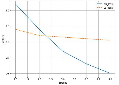
log.plot_epochs('trn_loss,val_loss'.split(','))

The plot of overall loss across training and validation data is as follows:

Now that we have trained a model, we will use it to predict on a new image in the next section.

Predict on a new image

In this section, we will leverage the model trained so far to predict and draw bounding boxes around objects and the corresponding class of object within the predicted bounding box on new images. The strategy we adopt is as follows:

1. Extract region proposals from the new image.
2. Resize and normalize each crop.

3. Feed-forward the processed crops to make predictions of class and the offsets.
4. Perform non-max suppression to fetch only those boxes that have the highest confidence of containing an object.

We execute the preceding strategy through a function that takes an image as input and a ground truth bounding box (this is used only so that we compare the ground truth and the predicted bounding box). We will continue coding from where we left off in the preceding section:

1. Define the test_predictions function to predict on a new image:

• The function takes filename as input:

def test_predictions(filename, show_output=True):

• Read the image and extract candidates:

    img = np.array(cv2.imread(filename, 1)[...,::-1])
    candidates = extract_candidates(img)
    candidates = [(x,y,x+w,y+h) for x,y,w,h in candidates]

• Loop through the candidates to resize and preprocess the image:

    input = []
    for candidate in candidates:
        x,y,X,Y = candidate
        crop = cv2.resize(img[y:Y,x:X], (224,224))
        input.append(preprocess_image(crop/255.)[None])
    input = torch.cat(input).to(device)

• Predict the class and offset:

    with torch.no_grad():
        rcnn.eval()
        probs, deltas = rcnn(input)
        probs = torch.nn.functional.softmax(probs, -1)
        confs, clss = torch.max(probs, -1)

• Extract the candidates that do not belong to the background class and sum up the candidates with the predicted bounding box offset values:

    candidates = np.array(candidates)
    confs,clss,probs,deltas =[tensor.detach().cpu().numpy() 
                                  for tensor in [confs, 
                                        clss, probs, deltas]]

    ixs = clss!=background_class
    confs, clss,probs,deltas,candidates = [tensor[ixs] for 
           tensor in [confs,clss, probs, deltas,candidates]]
    bbs = (candidates + deltas).astype(np.uint16)

• Use non-max suppression nms to eliminate near-duplicate bounding boxes (pairs of boxes that have an IoU greater than 0.05 are considered duplicates in this case). Among the duplicated boxes, we pick that box with the highest confidence and discard the rest:

    ixs = nms(torch.tensor(bbs.astype(np.float32)), 
                torch.tensor(confs), 0.05)
    confs,clss,probs,deltas,candidates,bbs = [tensor[ixs] 
                                            for tensor in 
                            [confs, clss, probs, deltas, 
                            candidates, bbs]]
    if len(ixs) == 1:
        confs, clss, probs, deltas, candidates, bbs = 
                [tensor[None] for tensor in [confs, clss,
                            probs, deltas, candidates, bbs]]

• Fetch the bounding box with the highest confidence:

    if len(confs) == 0 and not show_output:
        return (0,0,224,224), 'background', 0
    if len(confs) > 0:
        best_pred = np.argmax(confs)
        best_conf = np.max(confs)
        best_bb = bbs[best_pred]
        x,y,X,Y = best_bb

• Plot the image along with the predicted bounding box:

    _, ax = plt.subplots(1, 2, figsize=(20,10))
    show(img, ax=ax[0])
    ax[0].grid(False)
    ax[0].set_title('Original image')
    if len(confs) == 0:
        ax[1].imshow(img)
        ax[1].set_title('No objects')
        plt.show()
        return
    ax[1].set_title(target2label[clss[best_pred]])
    show(img, bbs=bbs.tolist(), 
        texts=[target2label[c] for c in clss.tolist()], 
        ax=ax[1], title='predicted bounding box and class')
    plt.show()
    return (x,y,X,Y),target2label[clss[best_pred]],best_conf

2. Execute the preceding function on a new image:

image, crops, bbs, labels, deltas, gtbbs, fpath = test_ds[7]
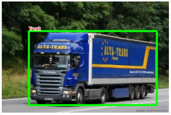
test_predictions(fpath)

The preceding code generates the following images:

From the preceding diagram, we can see that the prediction of the class of an image is accurate and the bounding box prediction is decent, too. Note that it took ~1.5 seconds to generate a prediction for the preceding image.

All of this time is consumed in generating region proposals, resizing each region proposal, passing them through a VGG backbone, and generating predictions using the defined model. Most of the time, however, is spent in passing each proposal through a VGG backbone. In the next section, we will learn about getting around this "passing each proposal to VGG" problem by using the Fast R-CNN architecture-based model.

Training Fast R-CNN-based custom object detectors

One of the major drawbacks of R-CNN is that it takes considerable time to generate predictions, as generating region proposals for each image, resizing the crops of regions, and extracting features corresponding to each crop (region proposal), constitute the bottleneck.

Fast R-CNN gets around this problem by passing the entire image through the pretrained model to extract features and then fetching the region of features that correspond to the region proposals (which are obtained from selectivesearch) of the original image. In the following sections, we will learn about the working details of Fast R-CNN before training it on our custom dataset.

Working details of Fast R-CNN

Let's understand Fast R-CNN through the following diagram:

Let's understand the preceding diagram through the following steps:

1. Pass the image through a pretrained model to extract features prior to the flattening layer; let's call the output as feature maps.
2. Extract region proposals corresponding to the image.
3. Extract the feature map area corresponding to the region proposals (note that when an image is passed through a VGG16 architecture, the image is downscaled by 32 at the output as there are 5 pooling operations performed. Thus, if a region exists with a bounding box of (40,32,200,240) in the original image, the feature map corresponding to the bounding box of (5,4,25,30) would correspond to the exact same region).
4. Pass the feature maps corresponding to region proposals through the RoI (Region of Interest) pooling layer one at a time so that all feature maps of region proposals have a similar shape. This is a replacement for the warping that was executed in the R-CNN technique.
5. Pass the RoI pooling layer output value through a fully connected layer.
6. Train the model to predict the class and offsets corresponding to each region proposal.

Now armed with an understanding of how Fast R-CNN works, in the next section, we will build the model using the same dataset that we leveraged in the R-CNN section.

Implementing Fast R-CNN for object detection on a custom dataset

In this section, we will work toward training our custom object detector using Fast R-CNN. Furthermore, so as to remain succinct, we provide only the additional or the changed code in this section (you should run all the code until step 2 in the Creating the training data sub-section in the previous section of R-CNN):

1. Create an FRCNNDataset class that returns images, labels, ground truths, region proposals, and the delta corresponding to each region proposal:

class FRCNNDataset(Dataset):
    def __init__(self, fpaths, rois, labels, deltas, gtbbs):
        self.fpaths = fpaths
        self.gtbbs = gtbbs
        self.rois = rois
        self.labels = labels
        self.deltas = deltas
    def __len__(self): return len(self.fpaths)
    def __getitem__(self, ix):
        fpath = str(self.fpaths[ix])
        image = cv2.imread(fpath, 1)[...,::-1]
        gtbbs = self.gtbbs[ix]
        rois = self.rois[ix]
        labels = self.labels[ix]
        deltas = self.deltas[ix]
        assert len(rois) == len(labels) == len(deltas), 
            f'{len(rois)}, {len(labels)}, {len(deltas)}'
        return image, rois, labels, deltas, gtbbs, fpath

    def collate_fn(self, batch):
        input, rois, rixs, labels, deltas = [],[],[],[],[]
        for ix in range(len(batch)):
            image, image_rois, image_labels, image_deltas, 
                image_gt_bbs, image_fpath = batch[ix]
            image = cv2.resize(image, (224,224))
            input.append(preprocess_image(image/255.)[None])
            rois.extend(image_rois)
            rixs.extend([ix]*len(image_rois))
            labels.extend([label2target[c] for c in 
                                image_labels])
            deltas.extend(image_deltas)
        input = torch.cat(input).to(device)
        rois = torch.Tensor(rois).float().to(device)
        rixs = torch.Tensor(rixs).float().to(device)
        labels = torch.Tensor(labels).long().to(device)
        deltas = torch.Tensor(deltas).float().to(device)
        return input, rois, rixs, labels, deltas

Note that the preceding code is very similar to what we have learned in the R-CNN section, with the only change being that we are returning more information (rois and rixs).

The rois matrix holds information regarding which RoI belongs to which image in the batch. Note that input contains multiple images, whereas rois is a single list of boxes. We wouldn't know how many rois belong to the first image and how many belong to the second image, and so on. This is where ridx comes into the picture. It is a list of indexes. Each integer in the list associates the corresponding bounding box with the appropriate image; for example, if ridx is [0,0,0,1,1,2,3,3,3], then we know the first three bounding boxes belong to the first image in the batch, and the next two belong to the second image in the batch.

2. Create training and test datasets:

n_train = 9*len(FPATHS)//10
train_ds = FRCNNDataset(FPATHS[:n_train], ROIS[:n_train], 
                        CLSS[:n_train], DELTAS[:n_train], 
                        GTBBS[:n_train])
test_ds = FRCNNDataset(FPATHS[n_train:], ROIS[n_train:], 
                       CLSS[n_train:], DELTAS[n_train:], 
                       GTBBS[n_train:])

from torch.utils.data import TensorDataset, DataLoader
train_loader = DataLoader(train_ds, batch_size=2, 
                          collate_fn=train_ds.collate_fn, 
                          drop_last=True)
test_loader = DataLoader(test_ds, batch_size=2, 
                         collate_fn=test_ds.collate_fn, 
                         drop_last=True)

3. Define a model to train on the dataset:

• First, import the RoIPool method present in the torchvision.ops class:

from torchvision.ops import RoIPool

• Define the FRCNN network module:

class FRCNN(nn.Module):
    def __init__(self):
        super().__init__()

• Load the pretrained model and freeze the parameters:

        rawnet = torchvision.models.vgg16_bn(pretrained=True)
        for param in rawnet.features.parameters():
            param.requires_grad = True

• Extract features until the last layer:

        self.seq = nn.Sequential(*list(
                            rawnet.features.children())[:-1])

• Specify that RoIPool is to extract a 7 x 7 output. Here, spatial_scale is the factor by which proposals (which come from the original image) need to be shrunk so that every output has the same shape prior to passing through the flatten layer. Images are 224 x 224 in size, while the feature map is 14 x 14 in size:

        self.roipool = RoIPool(7, spatial_scale=14/224)

• Define the output heads – cls_score and bbox:

        feature_dim = 512*7*7
        self.cls_score = nn.Linear(feature_dim, 
                                   len(label2target))
        self.bbox = nn.Sequential(
                          nn.Linear(feature_dim, 512),
                          nn.ReLU(),
                          nn.Linear(512, 4),
                          nn.Tanh(),
                        )

• Define the loss functions:

        self.cel = nn.CrossEntropyLoss()
        self.sl1 = nn.L1Loss()

• Define the forward method, which takes the image, region proposals, and the index of region proposals as input for the network defined earlier:

    def forward(self, input, rois, ridx):

• Pass the input image through the pretrained model:

        res = input
        res = self.seq(res)

• Create a matrix of rois as input for self.roipool, first by concatenating ridx as the first column and the next four columns being the absolute values of the region proposal bounding boxes:

        rois = torch.cat([ridx.unsqueeze(-1), rois*224], 
                            dim=-1)
        res = self.roipool(res, rois)
        feat = res.view(len(res), -1)
        cls_score = self.cls_score(feat)
        bbox=self.bbox(feat)#.view(-1,len(label2target),4)
        return cls_score, bbox

• Define the loss value calculation (calc_loss), just like we did in the R-CNN section:

    def calc_loss(self, probs, _deltas, labels, deltas):
        detection_loss = self.cel(probs, labels)
        ixs, = torch.where(labels != background_class)
        _deltas = _deltas[ixs]
        deltas = deltas[ixs]
        self.lmb = 10.0
        if len(ixs) > 0:
            regression_loss = self.sl1(_deltas, deltas)
            return detection_loss +
                self.lmb * regression_loss, 
                detection_loss.detach(), 
                regression_loss.detach()
        else:
            regression_loss = 0
            return detection_loss + 
                self.lmb * regression_loss, 
                detection_loss.detach(), 
                regression_loss

4. Define the functions to train and validate on a batch just like we did in the R-CNN section:

def train_batch(inputs, model, optimizer, criterion):
    input, rois, rixs, clss, deltas = inputs
    model.train()
    optimizer.zero_grad()
    _clss, _deltas = model(input, rois, rixs)
    loss, loc_loss, regr_loss = criterion(_clss, _deltas, 
                                           clss, deltas)
    accs = clss == decode(_clss)
    loss.backward()
    optimizer.step()
    return loss.detach(), loc_loss, regr_loss, 
        accs.cpu().numpy()
def validate_batch(inputs, model, criterion):
    input, rois, rixs, clss, deltas = inputs
    with torch.no_grad():
        model.eval()
        _clss,_deltas = model(input, rois, rixs)
        loss, loc_loss,regr_loss = criterion(_clss, _deltas, 
                                                clss, deltas)
        _clss = decode(_clss)
        accs = clss == _clss
    return _clss, _deltas,loss.detach(), loc_loss,regr_loss, 
        accs.cpu().numpy()

5. Define and train the model over increasing epochs:

frcnn = FRCNN().to(device)
criterion = frcnn.calc_loss
optimizer = optim.SGD(frcnn.parameters(), lr=1e-3)

n_epochs = 5
log = Report(n_epochs)
for epoch in range(n_epochs):

    _n = len(train_loader)
    for ix, inputs in enumerate(train_loader):
        loss, loc_loss,regr_loss, accs = train_batch(inputs, 
                                 frcnn, optimizer, criterion)
        pos = (epoch + (ix+1)/_n)
        log.record(pos, trn_loss=loss.item(), 
                   trn_loc_loss=loc_loss, 
                   trn_regr_loss=regr_loss, 
                   trn_acc=accs.mean(), end='
')
        
    _n = len(test_loader)
    for ix,inputs in enumerate(test_loader):
        _clss, _deltas, loss, 
        loc_loss, regr_loss, accs = validate_batch(inputs, 
                                          frcnn, criterion)
        pos = (epoch + (ix+1)/_n)
        log.record(pos, val_loss=loss.item(), 
                val_loc_loss=loc_loss, 
                val_regr_loss=regr_loss, 
                val_acc=accs.mean(), end='
')

# Plotting training and validation metrics
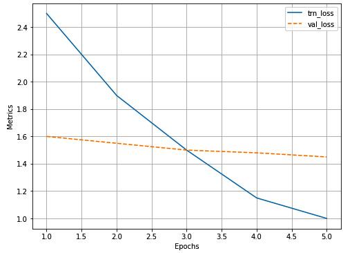
log.plot_epochs('trn_loss,val_loss'.split(','))

The variation in overall loss is as follows:

6. Define a function to predict on test images:

• Define the function that takes a filename as input and then reads the file and resizes it to 224 x 224:

import matplotlib.pyplot as plt
%matplotlib inline
import matplotlib.patches as mpatches
from torchvision.ops import nms
from PIL import Image
def test_predictions(filename):
    img = cv2.resize(np.array(Image.open(filename)), 
                               (224,224))

• Obtain region proposals and convert them to (x1,y1,x2,y2) format (top-left pixel and bottom-right pixel coordinates), and then convert these values to the ratio of width and height they are present in, in proportion to the image:

    candidates = extract_candidates(img)
    candidates = [(x,y,x+w,y+h) for x,y,w,h in candidates]

• Preprocess the image and scale the region of interests (rois):

    input = preprocess_image(img/255.)[None]
    rois = [[x/224,y/224,X/224,Y/224] for x,y,X,Y in 
                candidates]

• As all proposals belong to the same image, rixs will be a list of zeros (as many as the number of proposals):

    rixs = np.array([0]*len(rois))

• Forward propagate the input and rois through the trained model and get confidences and class scores for each proposal:

    rois,rixs = [torch.Tensor(item).to(device) for item in 
                    [rois, rixs]]
    with torch.no_grad():
        frcnn.eval()
        probs, deltas = frcnn(input, rois, rixs)
        confs, clss = torch.max(probs, -1)

• Filter out the background class:

    candidates = np.array(candidates)
    confs,clss,probs,deltas=[tensor.detach().cpu().numpy() 
                                  for tensor in [confs, 
                                       clss, probs, deltas]]
    
    ixs = clss!=background_class
    confs, clss, probs, deltas,candidates = [tensor[ixs] for 
           tensor in [confs, clss, probs, deltas,candidates]]
    bbs = candidates + deltas

• Remove near-duplicate bounding boxes with nms and get indices of those proposals in which the models that are highly confident are objects:

    ixs = nms(torch.tensor(bbs.astype(np.float32)), 
                torch.tensor(confs), 0.05)
    confs, clss, probs,deltas,candidates,bbs = [tensor[ixs] 
                            for tensor in [confs,clss,probs, 
                            deltas, candidates, bbs]]
    if len(ixs) == 1:
        confs, clss, probs, deltas, candidates, bbs = 
                    [tensor[None] for tensor in [confs,clss, 
                     probs, deltas, candidates, bbs]]
    
    bbs = bbs.astype(np.uint16)

• Plot the bounding boxes obtained:

    _, ax = plt.subplots(1, 2, figsize=(20,10))
    show(img, ax=ax[0])
    ax[0].grid(False)
    ax[0].set_title(filename.split('/')[-1])
    if len(confs) == 0:
        ax[1].imshow(img)
        ax[1].set_title('No objects')
        plt.show()
        return
    else:
        show(img,bbs=bbs.tolist(),texts=[target2label[c] for 
                                c in clss.tolist()],ax=ax[1])
        plt.show()

7. Predict on a test image:

test_predictions(test_ds[29][-1])

The preceding code results in the following:

The preceding code executes in 0.5 seconds, which is significantly better than that of R-CNN. However, it is still very slow to be used in real time. This is primarily because we are still using two different models, one to generate region proposals and another to make predictions of class and corrections. In the next chapter, we will learn about having a single model to make predictions, so that inference is quick in a real-time scenario.

Summary

In this chapter, we started with learning about creating a training dataset for the process of object localization and detection. Next, we learned about SelectiveSearch, a region proposal technique that recommends regions based on the similarity of pixels in proximity. We next learned about calculating the IoU metric to understand the goodness of the predicted bounding box around the objects present in the image. We next learned about performing non-max suppression to fetch one bounding box per object within an image before learning about building R-CNN and Fast R-CNN models from scratch. In addition, we learned about the reason why R-CNN is slow and how Fast R-CNN leverages RoI pooling and fetches region proposals from feature maps to make inference faster. Finally, we understood that having region proposals coming from a separate model is resulting in the higher time taken to predict on new images.

In the next chapter, we will learn about some of the modern object detection techniques that are used to make inference on a more real-time basis.

Questions

1. How does a region proposal technique generate proposals?
2. How is IoU calculated if there are multiple objects in an image?
3. Why does R-CNN take a long time to generate predictions?
4. Why is Fast R-CNN faster when compared with R-CNN?
5. How does RoI pooling work?
6. What is the impact of not having multiple layers post the feature map obtained when predicting the bounding box corrections?
7. Why do we have to assign a higher weight to regression loss when calculating overall loss?
8. How does non-max suppression work?