In the previous chapter, we learned that, as the number of images available in the training dataset increased, the classification accuracy of the model kept on increasing, to the extent where a training dataset comprising 8,000 images had a higher accuracy on validation dataset than a training dataset comprising 1,000 images. However, we do not always have the option of hundreds or thousands of images, along with the ground truths of their corresponding classes, in order to train a model. This is where transfer learning comes to the rescue.

Transfer learning is a technique where we transfer the learning of the model on a generic dataset to the specific dataset of interest. Typically, the pre-trained models used to perform transfer learning are trained on millions of images (which are generic and not the dataset of interest to us) and those pre-trained models are now fine-tuned to our dataset of interest.

In this chapter, we will learn about two different families of transfer learning architectures – variants of VGG architecture, and variants of ResNet architecture.

Along with understanding the architectures, we will also understand their application in two different use cases, age and gender classification, where we will learn about optimizing over both cross-entropy and mean absolute error losses at the same time, and facial key point detection, where we will learn about leveraging neural networks to generate multiple (136, instead of 1 prediction) continuous outputs in a single prediction. Finally, we will learn about a new library that assists in reducing code complexity considerably across the remaining chapters.

In summary, the following topics are covered in the chapter:

• Introducing transfer learning
• Understanding VGG16 and ResNet architectures
• Implementing facial key point detection
• Multi-task learning: Implementing age estimation and gender classification
• Introducing the torch_snippets library

Introducing transfer learning

Transfer learning is a technique where knowledge gained from one task is leveraged to solve another similar task.

Imagine a model that is trained on millions of images that span thousands of classes of objects (not just cats and dogs). The various filters (kernels) of the model would activate for a wide variety of shapes, colors, and textures within the images. Those filters can now be reused to learn features on a new set of images. Post learning the features, they can be connected to a hidden layer prior to the final classification layer for customizing on the new data.

ImageNet (http://www.image-net.org/) is a competition hosted to classify approximately 14 million images into 1,000 different classes. It has a variety of classes in the dataset, including Indian elephant, lionfish, hard disk, hair spray, and jeep.

The deep neural network architectures that we will go through in this chapter have been trained on the ImageNet dataset. Furthermore, given the variety and the volume of objects that are to be classified in ImageNet, the models are very deep so as to capture as much information as possible.

Let's understand the importance of transfer learning through a hypothetical scenario:

Consider a situation where we are working with images of a road, trying to classify them in terms of the objects they contain. Building a model from scratch might result in sub-optimal results, as the number of images could be insufficient to learn the various variations within the dataset (as we have seen in the previous use case, where training on 8,000 images resulted in a higher accuracy on a validation dataset than training on 2,000 images). A pre-trained model, trained on ImageNet, comes in handy in such a scenario. It would have already learned a lot about the traffic-related classes, such as cars, roads, trees, and humans, during training on the large ImageNet dataset. Hence, leveraging the already trained model would result in faster and more accurate training as the model already knows the generic shapes and now has to fit them for the specific images. With the intuition in place, let's now understand the high-level flow of transfer learning as follows:

1. Normalize the input images, normalized by the same mean and standard deviation that was used during the training of the pre-trained model.
2. Fetch the pre-trained model's architecture. Fetch the weights for this architecture that arose as a result of being trained on a large dataset.
3. Discard the last few layers of the pre-trained model.
4. Connect the truncated pre-trained model to a freshly initialized layer (or layers) where weights are randomly initialized. Ensure that the output of the last layer has as many neurons as the classes/outputs we would want to predict
5. Ensure that the weights of the pre-trained model are not trainable (in other words, frozen/not updated during backpropagation), but that the weights of the newly initialized layer and the weights connecting it to the output layer are trainable:

• We do not train the weights of the pre-trained model, as we assume those weights are already well learned for the task, and hence leverage the learning from a large model. In summary, we only learn the newly initialized layers for our small dataset.

6. Update the trainable parameters over increasing epochs to fit a model.

Now that we have an idea of how to implement transfer learning, let's understand the various architectures, how they are built, and the results when we apply transfer learning to the cats versus dogs use case in subsequent sections. First, we will cover in detail some of the various architectures that came out of VGG.

Understanding VGG16 architecture

VGG stands for Visual Geometry Group, which is based out of the University of Oxford, and 16 stands for the number of layers in the model. The VGG16 model is trained to classify objects in the ImageNet competition and stood as the runner-up architecture in 2014. The reason we are studying this architecture instead of the winning architecture (GoogleNet) is because of its simplicity and a larger acceptance in the vision community by using it in several other tasks. Let's understand the architecture of VGG16 along with how a VGG16 pre-trained model is accessible and represented in PyTorch.

1. Install the required packages:

import torchvision
import torch.nn as nn
import torch
import torch.nn.functional as F
from torchvision import transforms,models,datasets
!pip install torch_summary
from torchsummary import summary
device = 'cuda' if torch.cuda.is_available() else 'cpu'

The models module in the torchvision package hosts the various pre-trained models available in PyTorch.

2. Load the VGG16 model and register the model within the device:

model = models.vgg16(pretrained=True).to(device)

In the preceding code, we have called the vgg16 method within the models class. Furthermore, by mentioning pretrained = True, we are specifying that we load the weights that were used to classify images in the ImageNet competition, and then we are registering the model to the device.

3. Fetch the summary of the model:

summary(model, torch.zeros(1,3,224,224));

The output of the preceding code is as follows:

In the preceding summary, the 16 layers we mentioned are grouped as follows:

{1,2},{3,4,5},{6,7},{8,9,10},{11,12},{13,14},{15,16,17},{18,19},{20,21},{22,23,24},{25,26},{27,28},{29,30,31,32},{33,34,35},{36,37,38],{39}

The same summary can also be visualized thus:

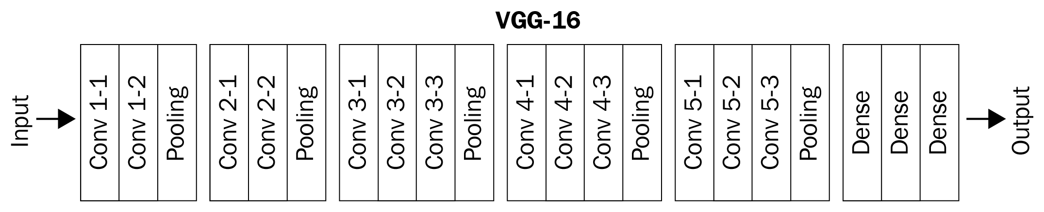
Note that there are ~138 million parameters (of which ~122 million are the linear layers at the end of the network – 102 + 16 + 4 million parameters) in this network, which comprises 13 layers of convolution and/or pooling, with increasing number of filters, and 3 linear layers.

Another way to understand the components of the VGG16 model is by simply printing it as follows:

model

This results in the following output:

Note that there are three major sub-modules in the model—features, avgpool, and classifier. Typically, we would freeze the features and avgpool modules. Delete the classifier module (or only a few layers at the bottom) and create a new one in its place that will predict the required number of classes corresponding to our dataset (instead of the existing 1,000).

Let's now understand how the VGG16 model is used in practice, using the cats versus dogs dataset (considering only 500 images in each class for training) in the following code:

1. Install the required packages:

import torch
import torchvision
import torch.nn as nn
import torch.nn.functional as F
from torchvision import transforms,models,datasets
import matplotlib.pyplot as plt
from PIL import Image
from torch import optim
device = 'cuda' if torch.cuda.is_available() else 'cpu'
import cv2, glob, numpy as np, pandas as pd
from glob import glob
import torchvision.transforms as transforms
from torch.utils.data import DataLoader, Dataset

2. Download the dataset and specify the training and test directories:

• Download the dataset. Assuming that we are working on Google Colab, we perform the following steps, where we provide the authentication key and place it in a location where Kaggle can use the key to authenticate us and download the dataset:

!pip install -q kaggle
from google.colab import files
files.upload()
!mkdir -p ~/.kaggle
!cp kaggle.json ~/.kaggle/
!ls ~/.kaggle
!chmod 600 /root/.kaggle/kaggle.json

• Download the dataset and unzip it:

!kaggle datasets download -d tongpython/cat-and-dog
!unzip cat-and-dog.zip

• Specify the training and test image folders:

train_data_dir = 'training_set/training_set'
test_data_dir = 'test_set/test_set'

3. Provide the class that returns input-output pairs for the cats and dogs dataset, just like we did in Chapter 4, Introducing Convolutional Neural Networks. Note that, in this case, we are fetching the first 500 images only from each folder:

class CatsDogs(Dataset):
    def __init__(self, folder):
        cats = glob(folder+'/cats/*.jpg')
        dogs = glob(folder+'/dogs/*.jpg')
        self.fpaths = cats[:500] + dogs[:500]
        self.normalize = transforms.Normalize(mean=[0.485, 
                   0.456, 0.406],std=[0.229, 0.224, 0.225])
        from random import shuffle, seed; seed(10); 
        shuffle(self.fpaths)
        self.targets =[fpath.split('/')[-1].startswith('dog') 
                        for fpath in self.fpaths] 
    def __len__(self): return len(self.fpaths)
    def __getitem__(self, ix):
        f = self.fpaths[ix]
        target = self.targets[ix]
        im = (cv2.imread(f)[:,:,::-1])
        im = cv2.resize(im, (224,224))
        im = torch.tensor(im/255)
        im = im.permute(2,0,1)
        im = self.normalize(im) 
        return im.float().to(device), 
            torch.tensor([target]).float().to(device)

The main difference between the cats_dogs class in this section and in chapter 4 is the normalize function that we are applying using the Normalize function from the transforms module.

4. Fetch the images and their labels:

data = CatsDogs(train_data_dir)

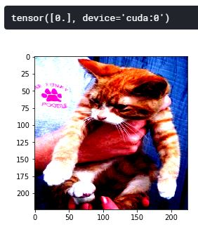
Let's now inspect a sample image and its corresponding class:

im, label = data[200]
plt.imshow(im.permute(1,2,0).cpu())
print(label)

The preceding code results in the following output:

5. Define the model. Download the pre-trained VGG16 weights and then freeze the features module and train using the avgpool and classifier modules:

• First, we download the pretrained VGG16 model from the models class:

def get_model():
    model = models.vgg16(pretrained=True)

• Specify that we want to freeze all the parameters in the model downloaded previously:

    for param in model.parameters():
        param.requires_grad = False

In the preceding code, we are freezing parameter updates during backpropagation by specifying param.requires_grad = False.

• Replace the avgpool module to return a feature map of size 1 x 1 instead of 7 x 7, in other words, the output is now going to be batch_size x 512 x 1 x 1:

    model.avgpool = nn.AdaptiveAvgPool2d(output_size=(1,1))

• Define the classifier module of the model, where we first flatten the output of the avgpool module, connect the 512 units to the 128 units, and perform an activation prior to connecting to the output layer:

    model.classifier = nn.Sequential(nn.Flatten(),
                                    nn.Linear(512, 128),
                                    nn.ReLU(),
                                    nn.Dropout(0.2),
                                    nn.Linear(128, 1),
                                    nn.Sigmoid())

• Define the loss function (loss_fn), optimizer, and return them along with the defined model:

    loss_fn = nn.BCELoss()
    optimizer = torch.optim.Adam(model.parameters(),lr= 1e-3)
    return model.to(device), loss_fn, optimizer

Note that in the preceding code, we have first frozen all the parameters of the pre-trained model and have then overwritten the avgpool and classifier modules. Now, the rest of the code is going to look similar to what we have seen in the previous chapter.

A summary of the model is as follows:

!pip install torch_summary
from torchsummary import summary
model, criterion, optimizer = get_model()
summary(model, torch.zeros(1,3,224,224))

The preceding code results in the following output:

6. Define a function to train on a batch, calculate accuracy, and to get data just like we did in Chapter 4, Introducing Convolutional Neural Networks:

• Train on a batch of data:

def train_batch(x, y, model, opt, loss_fn):
    model.train()
    prediction = model(x)
    batch_loss = loss_fn(prediction, y)
    batch_loss.backward()
    optimizer.step()
    optimizer.zero_grad()
    return batch_loss.item()

• Define a function to calculate accuracy on a batch of data:

@torch.no_grad()
def accuracy(x, y, model):
    model.eval()
    prediction = model(x)
    is_correct = (prediction > 0.5) == y
    return is_correct.cpu().numpy().tolist()

• Define a function to fetch the data loaders:

def get_data():
    train = CatsDogs(train_data_dir)
    trn_dl = DataLoader(train, batch_size=32, shuffle=True, 
                            drop_last = True)
    val = CatsDogs(test_data_dir)
    val_dl = DataLoader(val, batch_size=32, shuffle=True, 
                            drop_last = True)
    return trn_dl, val_dl

• Initialize the get_data and get_model functions:

trn_dl, val_dl = get_data()
model, loss_fn, optimizer = get_model()

7. Train the model over increasing epochs, just like we did in Chapter 4, Introducing Convolutional Neural Networks:

train_losses, train_accuracies = [], []
val_accuracies = []
for epoch in range(5):
    print(f" epoch {epoch + 1}/5")
    train_epoch_losses, train_epoch_accuracies = [], []
    val_epoch_accuracies = []

    for ix, batch in enumerate(iter(trn_dl)):
        x, y = batch
        batch_loss = train_batch(x, y, model, optimizer, 
                                        loss_fn)
        train_epoch_losses.append(batch_loss) 
    train_epoch_loss = np.array(train_epoch_losses).mean()

    for ix, batch in enumerate(iter(trn_dl)):
        x, y = batch
        is_correct = accuracy(x, y, model)
        train_epoch_accuracies.extend(is_correct)
    train_epoch_accuracy = np.mean(train_epoch_accuracies)

    for ix, batch in enumerate(iter(val_dl)):
        x, y = batch
        val_is_correct = accuracy(x, y, model)
        val_epoch_accuracies.extend(val_is_correct)
    val_epoch_accuracy = np.mean(val_epoch_accuracies)

    train_losses.append(train_epoch_loss)
    train_accuracies.append(train_epoch_accuracy)
    val_accuracies.append(val_epoch_accuracy)

8. Plot the training and test accuracy values over increasing epochs:

epochs = np.arange(5)+1
import matplotlib.ticker as mtick
import matplotlib.pyplot as plt
import matplotlib.ticker as mticker
%matplotlib inline
plt.plot(epochs, train_accuracies, 'bo', 
         label='Training accuracy')
plt.plot(epochs, val_accuracies, 'r', 
         label='Validation accuracy')
plt.gca().xaxis.set_major_locator(mticker.MultipleLocator(1))
plt.title('Training and validation accuracy 
with VGG16 
and 1K training data points')
plt.xlabel('Epochs')
plt.ylabel('Accuracy')
plt.ylim(0.95,1)
plt.gca().set_yticklabels(['{:.0f}%'.format(x*100) 
                           for x in plt.gca().get_yticks()]) 
plt.legend()
plt.grid('off')
plt.show()

This results in the following output:

Note that we are able to get an accuracy of 98% within the first epoch, even on a small dataset of 1,000 images (500 images of each class).

The training and validation accuracy when we use VGG11 and VGG19 in place of the VGG16 pre-trained model is as follows:

Note that, while the VGG19-based model has slightly better accuracy than that of a VGG16-based model with an accuracy of 98% on validation data, the VGG11-based model has a slightly lower accuracy of 97%.

From VGG16 to VGG19, we have increased the number of layers, and generally, the deeper the neural network, the better its accuracy.

However, if merely increasing the number of layers is the trick, then we could keep on adding more layers (while taking care to avoid overfitting) to the model to get more accurate results on ImageNet and then fine-tune it for a dataset of interest. Unfortunately, that does not turn out to be true.

There are multiple reasons why it is not that easy. Any of the following are likely to happen as we go deeper in terms of architecture:

• We have to learn a larger number of features.
• Vanishing gradients arise.
• There is too much information modification at deeper layers.

ResNet comes into the picture to address this specific scenario of identifying when not to learn, which we will learn about in the next section.

Understanding ResNet architecture

While building too deep a network, there are two problems. In forward propagation, the last few layers of the network have almost no information about what the original image was. In backpropagation, the first few layers near the input hardly get any gradient updates due to vanishing gradients (in other words, they are almost zero). To solve both problems, residual networks (ResNet) use a highway-like connection that transfers raw information from the previous few layers to the later layers. In theory, even the last layer will have the entire information of the original image due to this highway network. And because of the skipping layers, the backward gradients will flow freely to the initial layers with little modification.

The term residual in the residual network is the additional information that the model is expected to learn from the previous layer that needs to be passed on to the next layer.

A typical residual block appears as follows:

As you can see, while so far, we have been interested in extracting the F(x) value, where x is the value coming from the previous layer, in the case of a residual network, we are extracting not only the value after passing through the weight layers, which is F(x), but are also summing up F(x) with the original value, which is x.

So far, we have been using standard layers that performed either linear or convolution transformations F(x) along with some non-linear activation. Both of these operations in some sense destroy the input information. For the first time, we are seeing a layer that not only transforms the input, but also preserves it, by adding the input directly to the transformation – F(x) + x. This way, in certain scenarios, the layer has very little burden in remembering what the input is, and can focus on learning the correct transformation for the task.

Let's have a more detailed look at the residual layer through code by building a residual block:

1. Define a class with the convolution operation (weight layer in the previous diagram) in the __init__ method:

class ResLayer(nn.Module):
     def __init__(self,ni,no,kernel_size,stride=1):
        super(ResLayer, self).__init__()
        padding = kernel_size - 2
        self.conv = nn.Sequential(
                        nn.Conv2d(ni, no, kernel_size, stride, 
                                  padding=padding),
                        nn.ReLU()
                    )

Note that, in the preceding code, we defined padding as the dimension of the output when passed through convolution, and the dimension of the input should remain the same if we were to sum the two.

2. Define the forward method:

     def forward(self, x):
         x = self.conv(x) + x
         return x

In the preceding code, we are getting an output that is a sum of the input passed through the convolution operations and the original input.

Now that we have learned about how residual blocks work, let's understand how the residual blocks are connected in a pre-trained, residual block-based network, ResNet18:

As you can see, there are 18 layers in the architecture, hence it is referred to as a ResNet18 architecture. Furthermore, notice how the skip connections are made across the network. It is not made at every convolution layer, but after every two layers instead.

Now that we understand the composition of a ResNet architecture, let's build a model based on ResNet18 architecture to classify between dogs and cats, just like we did in the previous section using VGG16.

To build a classifier, the code up to step 3 of the VGG16 section remains the same as it deals with importing packages, fetching data, and inspecting them. So, we will start by understanding the composition of a pre-trained ResNet18 model:

1. Load the pre-trained ResNet18 model and inspect the modules within the loaded model:

model = models.resnet18(pretrained=True).to(device)
model

The structure of the ResNet18 model contains the following components:

• Convolution
• Batch normalization
• ReLU
• MaxPooling
• Four layers of ResNet blocks
• Average pooling (avgpool)
• A fully connected layer (fc)

As we have done in VGG16, we will freeze all the different modules, but update the parameters in the avgpool and fc modules in the next step.

2. Define the model architecture, loss function, and optimizer:

def get_model():
    model = models.resnet18(pretrained=True)
    for param in model.parameters():
        param.requires_grad = False
    model.avgpool = nn.AdaptiveAvgPool2d(output_size=(1,1))
    model.fc = nn.Sequential(nn.Flatten(),
    nn.Linear(512, 128),
    nn.ReLU(),
    nn.Dropout(0.2),
    nn.Linear(128, 1),
    nn.Sigmoid())
    loss_fn = nn.BCELoss()
    optimizer = torch.optim.Adam(model.parameters(),lr= 1e-3)
    return model.to(device), loss_fn, optimizer

In the preceding model, the input shape of the fc module is 512, as the output of avgpool has the shape of batch size x 512 x 1 x 1.

Now that we have defined the model, let's execute steps 5 and 6 as per the VGG section. The variation in training and validation accuracies after training the model (where the model is ResNet18, ResNet34, ResNet50, ResNet101, and ResNet152 for each of the following charts) over increasing epochs is as follows:

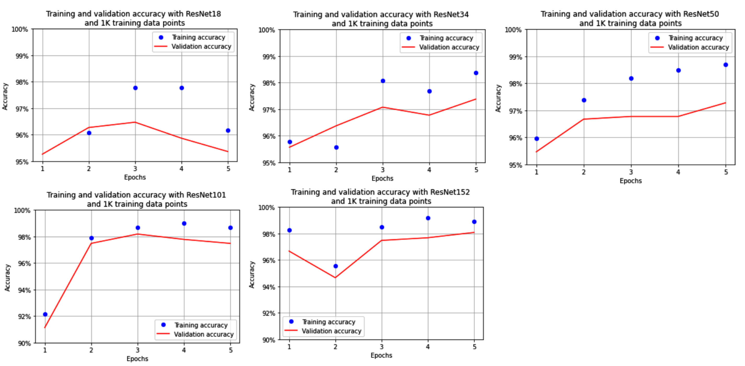
We see that the accuracy of the model, when trained on only 1,000 images, varies between 97% and 98%, where accuracy increases with an increase in the number of layers in ResNet.

Now that we have learned about leveraging pre-trained models to predict for a class that is binary, in the next sections, we will learn about leveraging pre-trained models to solve real-world use cases that involve the following:

• Multi-regression: Prediction of multiple values given an image as input – facial key point detection
• Multi-task learning: Prediction of multiple items in a single shot – age estimation and gender classification

Implementing facial key point detection

So far, we have learned about predicting classes that are binary (cats versus dogs) or are multi-label (fashionMNIST). Let's now learn a regression problem and, in so doing, a task where we are predicting not one but several continuous outputs. Imagine a scenario where you are asked to predict the key points present on an image of a face, for example, the location of the eyes, nose, and chin. In this scenario, we need to employ a new strategy to build a model to detect the key points.

Before we dive further, let's understand what we are trying to achieve through the following image:

As you can observe in the preceding image, facial key points denote the markings of various key points on the image that contains a face.

To solve this problem, we would have to solve a few problems first:

• Images can be of different shapes:
• This warrants an adjustment in the key point locations while adjusting images to bring them all to a standard image size.
• Facial key points are similar to points on a scatter plot, but scattered based on a certain pattern this time:
• This means that the values are anywhere between 0 and 224 if the image is resized to a shape of 224 x 224 x 3.
• Normalize the dependent variable (the location of facial key points) as per the size of the image:
• The key point values are always between 0 and 1 if we consider their location relative to image dimensions.
• Given that the dependent variable values are always between o and 1, we can use a sigmoid layer at the end to fetch values that will be between 0 and 1.

Let's formulate the pipeline of solving this use case:

1. Import the relevant packages.
2. Import data.
3. Define the class that prepares the dataset:

• Ensure appropriate pre-processing is done on input images to perform transfer learning.
• Ensure that the location of key points is processed in such a way that we fetch their relative position with respect to the processed image.

4. Define the model, loss function, and optimizer:

• The loss function is the mean absolute error, as the output is a continuous value between 0 and 1.

5. Train the model over increasing epochs.

Let's now implement the preceding steps:

1. Import the relevant packages and the dataset:

import torchvision
import torch.nn as nn
import torch
import torch.nn.functional as F
from torchvision import transforms, models, datasets
from torchsummary import summary
import numpy as np, pandas as pd, os, glob, cv2
from torch.utils.data import TensorDataset,DataLoader,Dataset
from copy import deepcopy
from mpl_toolkits.mplot3d import Axes3D
import matplotlib.pyplot as plt
%matplotlib inline
from sklearn import cluster
device = 'cuda' if torch.cuda.is_available() else 'cpu'

2. Download and import the relevant data. You can download the relevant data that contains images and their corresponding facial key points:

!git clone https://github.com/udacity/P1_Facial_Keypoints.git
!cd P1_Facial_Keypoints
root_dir = 'P1_Facial_Keypoints/data/training/'
all_img_paths = glob.glob(os.path.join(root_dir, '*.jpg'))
data = pd.read_csv(
    'P1_Facial_Keypoints/data/training_frames_keypoints.csv')

A sample of the imported dataset is as follows:

In the preceding output, column 1 represents the name of the image, even columns represent the x-axis value corresponding to each of the 68 key points of the face, and the rest of the odd columns (except the first column) represent the y-axis value corresponding to each of the 68 key points.

3. Define the FacesData class that provides input and output data points for the data loader:

class FacesData(Dataset):

• Now let's define the __init__ method, which takes the data frame of the file (df) as input:

    def __init__(self, df):
        super(FacesData).__init__()
        self.df = df

• Define the mean and standard deviation with which images are to be pre-processed so that they can be consumed by the pre-trained VGG16 model:

        self.normalize = transforms.Normalize(
                                mean=[0.485, 0.456, 0.406], 
                                std=[0.229, 0.224, 0.225])

• Now, define the __len__ method:

    def __len__(self): return len(self.df)

Next, we define the __getitem__ method, where we fetch the image corresponding to a given index, scale it, fetch the key point values corresponding to the given index, normalize the key points so that we have the location of the key points as a proportion of the size of the image, and pre-process the image.

• Define the __getitem__ method and fetch the path of the image corresponding to a given index (ix):

    def __getitem__(self, ix):
        img_path = 'P1_Facial_Keypoints/data/training/' +  
                                        self.df.iloc[ix,0]

• Scale the image:

        img = cv2.imread(img_path)/255.

• Normalize the expected output values (key points) as a proportion of the size of the original image:

        kp = deepcopy(self.df.iloc[ix,1:].tolist())
        kp_x = (np.array(kp[0::2])/img.shape[1]).tolist()
        kp_y = (np.array(kp[1::2])/img.shape[0]).tolist()

In the preceding code, we are ensuring that key points are provided as a proportion of the original image's size. This is done so that when we resize the original image, the location of the key points is not changed, as the key points are provided as a proportion of the original image. Furthermore, by getting key points as a proportion of the original image, we have expected output values that are between 0 and 1.

• Return the key points (kp2) and image (img) after pre-processing the image:

        kp2 = kp_x + kp_y
        kp2 = torch.tensor(kp2) 
        img = self.preprocess_input(img)
        return img, kp2

• Define the function to pre-process an image (preprocess_input):

    def preprocess_input(self, img):
        img = cv2.resize(img, (224,224))
        img = torch.tensor(img).permute(2,0,1)
        img = self.normalize(img).float()
        return img.to(device)

• Define a function to load the image, which will be useful when we want to visualize a test image and the predicted key points of the test image:

    def load_img(self, ix):
        img_path = 'P1_Facial_Keypoints/data/training/' + 
                                        self.df.iloc[ix,0]
        img = cv2.imread(img_path)
        img = cv2.cvtColor(img, cv2.COLOR_BGR2RGB)/255.
        img = cv2.resize(img, (224,224))
        return img

4. Let's now create a training and test data split and establish training and test datasets and data loaders:

from sklearn.model_selection import train_test_split

train, test = train_test_split(data, test_size=0.2, 
                                random_state=101)
train_dataset = FacesData(train.reset_index(drop=True))
test_dataset = FacesData(test.reset_index(drop=True))

train_loader = DataLoader(train_dataset, batch_size=32)
test_loader = DataLoader(test_dataset, batch_size=32)

In the preceding code, we have split the training and test datasets by person name in the input data frame and fetched their corresponding objects.

5. Let's now define the model that we will leverage to identify key points in an image:

• Load the pre-trained VGG16 model:

def get_model():
    model = models.vgg16(pretrained=True)

• Ensure that the parameters of the pre-trained model are frozen first:

    for param in model.parameters():
        param.requires_grad = False

Overwrite and unfreeze the parameters of the last two layers of the model:

    model.avgpool = nn.Sequential( nn.Conv2d(512,512,3),
                                      nn.MaxPool2d(2),
                                      nn.Flatten())
    model.classifier = nn.Sequential(
                                      nn.Linear(2048, 512),
                                      nn.ReLU(),
                                      nn.Dropout(0.5),
                                      nn.Linear(512, 136),
                                      nn.Sigmoid()
                                    )

Note that the last layer of the model in the classifier module is a sigmoid function that returns a value between o and 1 and that the expected output will always be between 0 and 1 as keypoint locations are a fraction of the original image's dimensions:

• Define the loss function and optimizer and return them along with the model:

    criterion = nn.L1Loss()
    optimizer = torch.optim.Adam(model.parameters(), lr=1e-4)
    return model.to(device), criterion, optimizer

Note that the loss function is L1Loss, in other words, we are performing mean absolute error reduction on the prediction of the location of facial key points (which will be predicted as a percentage of the image's width and height).

6. Get the model, loss function, and the corresponding optimizer:

model, criterion, optimizer = get_model()

7. Define functions to train on a batch of data points and also to validate on the test dataset:

• Training a batch, as we have done earlier, involves fetching the output of passing input through the model, calculating the loss value, and performing backpropagation to update the weights:

def train_batch(img, kps, model, optimizer, criterion):
    model.train()
    optimizer.zero_grad()
    _kps = model(img.to(device))
    loss = criterion(_kps, kps.to(device))
    loss.backward()
    optimizer.step()
    return loss

• Build a function that returns the loss on test data and the predicted key points:

def validate_batch(img, kps, model, criterion):
    model.eval()
    with torch.no_grad(): 
        _kps = model(img.to(device))
    loss = criterion(_kps, kps.to(device))
    return _kps, loss

8. Train the model based on training the data loader and test it on test data, as we have done hitherto in previous sections:

train_loss, test_loss = [], []
n_epochs = 50

for epoch in range(n_epochs):
    print(f" epoch {epoch+ 1} : 50")
    epoch_train_loss, epoch_test_loss = 0, 0
    for ix, (img,kps) in enumerate(train_loader):
        loss = train_batch(img, kps, model, optimizer, 
                                criterion)
        epoch_train_loss += loss.item() 
    epoch_train_loss /= (ix+1)

    for ix,(img,kps) in enumerate(test_loader):
        ps, loss = validate_batch(img, kps, model, criterion)
        epoch_test_loss += loss.item() 
    epoch_test_loss /= (ix+1)

    train_loss.append(epoch_train_loss)
    test_loss.append(epoch_test_loss)

9. Plot the training and test loss over increasing epochs:

epochs = np.arange(50)+1
import matplotlib.ticker as mtick
import matplotlib.pyplot as plt
import matplotlib.ticker as mticker
%matplotlib inline
plt.plot(epochs, train_loss, 'bo', label='Training loss')
plt.plot(epochs, test_loss, 'r', label='Test loss')
plt.title('Training and Test loss over increasing epochs')
plt.xlabel('Epochs')
plt.ylabel('Loss')
plt.legend()
plt.grid('off')
plt.show()

The preceding code results in the following output:

10. Test our model on a random test image's index, let's say 0. Note that in the following code, we are leveraging the load_img method in the FacesData class that was created earlier:

ix = 0
plt.figure(figsize=(10,10))
plt.subplot(221)
plt.title('Original image')
im = test_dataset.load_img(ix)
plt.imshow(im)
plt.grid(False)
plt.subplot(222)
plt.title('Image with facial keypoints')
x, _ = test_dataset[ix]
plt.imshow(im)
kp = model(x[None]).flatten().detach().cpu()
plt.scatter(kp[:68]*224, kp[68:]*224, c='r')
plt.grid(False)
plt.show()

The preceding code results in the following output:

From the preceding image, we see that the model is able to identify the facial key points fairly accurately, given the image as an input.

In this section, we have built the facial key point detector model from scratch. However, there are pre-trained models that are built both for 2D and 3D point detection. In the next section, we will learn about leveraging the face alignment library to fetch 2D and 3D key points of a face.

2D and 3D facial key point detection

In this section, we will leverage a pre-trained model that can detect the 2D and 3D key points present in a face in a few lines of code.

To work on this, we will leverage the face-alignment library:

1. Install the required packages:

!pip install -qU face-alignment
import face_alignment, cv2

2. Import the image:

!wget https://www.dropbox.com/s/2s7xjto7rb6q7dc/Hema.JPG

3. Define the face alignment method, where we specify whether we want to fetch key point landmarks in 2D or 3D:

fa = face_alignment.FaceAlignment(
                    face_alignment.LandmarksType._2D, 
                    flip_input=False, device='cpu')

4. Read the input image and provide it to the get_landmarks method:

input = cv2.imread('Hema.JPG')
preds = fa.get_landmarks(input)[0]
print(preds.shape)
# (68,2)

In the preceding lines of code, we are leveraging the get_landmarks method in the fa class to fetch the 68 x and y coordinates corresponding to the facial key points.

5. Plot the image with the detected key points:

import matplotlib.pyplot as plt
%matplotlib inline
fig,ax = plt.subplots(figsize=(5,5))
plt.imshow(cv2.cvtColor(cv2.imread('Hema.JPG'), 
                        cv2.COLOR_BGR2RGB))
ax.scatter(preds[:,0], preds[:,1], marker='+', c='r')
plt.show()

The preceding code results in the following output:

Notice the scatter plot of + symbols around the 60 possible facial key points.

In a similar manner, the 3D projections of facial key points are obtained as follows:

fa = face_alignment.FaceAlignment(
                        face_alignment.LandmarksType._3D, 
                        flip_input=False, device='cpu')
input = cv2.imread('Hema.JPG')
preds = fa.get_landmarks(input)[0]
import pandas as pd
df = pd.DataFrame(preds)
df.columns = ['x','y','z']
import plotly.express as px
fig = px.scatter_3d(df, x = 'x', y = 'y', z = 'z')
fig.show()

Note that the only change from the code used in the 2D key points scenario is that we specified LandmarksType to be 3D in place of 2D

The preceding code results in the following output:

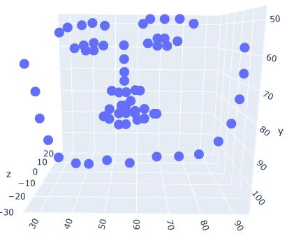
With the code leveraging the face_alignment library, we see that we are able to leverage the pre-trained facial key point detection models to have high accuracy in predicting on new images.

So far, across different use cases, we have learned the following:

• Cats versus dogs: Predicting for binary classification
• FashionMNIST: Predicting for a label among 10 possible classes
• Facial key points: Predicting multiple values between 0 and 1 for a given image

In the next section, we will learn about predicting a binary class and a regression value together in a single shot using a single network.

Multi-task learning – Implementing age estimation and gender classification

Multi-task learning is a branch of research where a single/few inputs are used to predict several different but ultimately connected outputs. For example, in a self-driving car, the model needs to identify obstacles, plan routes, give the right amount of throttle/brake and steering, to name but a few. It needs to do all of these in a split second by considering the same set of inputs (which would come from several sensors)

From the various use cases we have solved so far, we are in a position to train a neural network and estimate the age of a person given an image or predict the gender of the person given an image, separately, one task at a time. However, we have not looked at a scenario where we will be able to predict both age and gender in a single shot from an image. Predicting two different attributes in a single shot is important, as the same image is used for both predictions (this will be further appreciated as we perform object detection in Chapter 7, Basics of Object Detection).

In this section, we will learn about predicting both attributes, continuous and categorical predictions, in a single forward pass.

The strategy we adopt is as follows:

1. Import the relevant packages.
2. Fetch a dataset that contains images of persons, their gender, and age information.
3. Create training and test datasets by performing appropriate pre-processing.
4. Build a model where the following applies:

• All the layers of the model remain similar to the models we have built so far, except for the last part.
• In the last part, create two separate layers branching out from the preceding layer, where one layer corresponds to age estimation and the other to gender classification.
• Ensure that you have different loss functions for each branch of output, as age is a continuous value (requiring an mse or mae loss calculation) and gender is a categorical value (requiring a cross-entropy loss calculation).
• Take a weighted summation of age estimation loss and gender classification loss.
• Minimize the overall loss by performing backpropagation that optimizes weight values.

5. Train model and predict on new images.

With the preceding strategy in place, let's code up the use case:

1. Import the relevant packages:

import torch
import numpy as np, cv2, pandas as pd, glob, time
import matplotlib.pyplot as plt
%matplotlib inline
import torch.nn as nn
from torch import optim
import torch.nn.functional as F
from torch.utils.data import Dataset, DataLoader
import torchvision
from torchvision import transforms, models, datasets
device = 'cuda' if torch.cuda.is_available() else 'cpu'

2. Fetch the dataset:

from pydrive.auth import GoogleAuth
from pydrive.drive import GoogleDrive
from google.colab import auth
from oauth2client.client import GoogleCredentials

auth.authenticate_user()
gauth = GoogleAuth()
gauth.credentials=GoogleCredentials.get_application_default()
drive = GoogleDrive(gauth)

def getFile_from_drive( file_id, name ):
    downloaded = drive.CreateFile({'id': file_id})
    downloaded.GetContentFile(name)

getFile_from_drive('1Z1RqRo0_JiavaZw2yzZG6WETdZQ8qX86', 
                   'fairface-img-margin025-trainval.zip')
getFile_from_drive('1k5vvyREmHDW5TSM9QgB04Bvc8C8_7dl-', 
                   'fairface-label-train.csv')
getFile_from_drive('1_rtz1M1zhvS0d5vVoXUamnohB6cJ02iJ', 
                   'fairface-label-val.csv')

!unzip -qq fairface-img-margin025-trainval.zip

3. The dataset we downloaded can be loaded and is structured in the following way:

trn_df = pd.read_csv('fairface-label-train.csv')
val_df = pd.read_csv('fairface-label-val.csv')
trn_df.head()

The preceding code results in the following output:

4. Build the GenderAgeClass class that takes a filename as input and returns the corresponding image, gender, and scaled age. We scale age as it is a continuous number and, as we have seen in Chapter 3, Building a Deep Neural Network with PyTorch, it is better to scale data to avoid vanishing gradients and then rescale it during post-processing:

• Provide file paths (fpaths) of images in the __init__ method:

IMAGE_SIZE = 224
class GenderAgeClass(Dataset):
    def __init__(self, df, tfms=None):
        self.df = df
        self.normalize = transforms.Normalize(
                                mean=[0.485, 0.456, 0.406], 
                                std=[0.229, 0.224, 0.225])

• Define the __len__ method as the one that returns the number of images in the input:

    def __len__(self): return len(self.df)

• Define the __getitem__ method that fetches information of an image at a given position, ix:

    def __getitem__(self, ix):
        f = self.df.iloc[ix].squeeze()
        file = f.file
        gen = f.gender == 'Female'
        age = f.age
        im = cv2.imread(file)
        im = cv2.cvtColor(im, cv2.COLOR_BGR2RGB)
        return im, age, gen

• Write a function that pre-processes an image, which involves resizing the image, permuting the channels, and performing normalization on a scaled image:

    def preprocess_image(self, im):
        im = cv2.resize(im, (IMAGE_SIZE, IMAGE_SIZE))
        im = torch.tensor(im).permute(2,0,1)
        im = self.normalize(im/255.)
        return im[None]

• Create the collate_fn method, which fetches a batch of data where the data points are pre-processed as follows:
• Process each image using the process_image method.
• Scale the age by 80 (the maximum age value present in the dataset), so that all values are between 0 and 1.
• Convert gender to a float value.
• Image, age, and gender are each converted into torch objects and returned:

    def collate_fn(self, batch):
        'preprocess images, ages and genders'
        ims, ages, genders = [], [], []
        for im, age, gender in batch:
            im = self.preprocess_image(im)
            ims.append(im)

            ages.append(float(int(age)/80))
            genders.append(float(gender))

        ages, genders = [torch.tensor(x).to(device).float() 
                            for x in [ages, genders]]
        ims = torch.cat(ims).to(device)

        return ims, ages, genders

5. We now define the training and validation datasets and data loaders:

• Create the datasets:

trn = GenderAgeClass(trn_df)
val = GenderAgeClass(val_df)

• Specify the data loaders:

device = 'cuda' if torch.cuda.is_available() else 'cpu'
train_loader = DataLoader(trn, batch_size=32, shuffle=True, 
                    drop_last=True,collate_fn=trn.collate_fn)
test_loader = DataLoader(val, batch_size=32, 
                         collate_fn=val.collate_fn)
a,b,c, = next(iter(train_loader))
print(a.shape, b.shape, c.shape)

6. Define the model, loss function, and optimizer:

• First, in the function, we load the pre-trained VGG16 model:

def get_model():
    model = models.vgg16(pretrained = True)

• Next, freeze the loaded model (by specifying param.requires_grad = False):

    for param in model.parameters():
        param.requires_grad = False

• Overwrite the avgpool layer with our own layer:

    model.avgpool = nn.Sequential(
                        nn.Conv2d(512,512, kernel_size=3),
                        nn.MaxPool2d(2),
                        nn.ReLU(),
                        nn.Flatten()
                    )

Now comes the key part. We deviate from what we have learned so far by creating two branches of outputs. This is performed as follows:

• Build a neural network class named ageGenderClassifier with the following in the __init__ method:

    class ageGenderClassifier(nn.Module):
        def __init__(self):
            super(ageGenderClassifier, self).__init__()

• Define the intermediate layer calculations:

            self.intermediate = nn.Sequential(
                                    nn.Linear(2048,512),
                                    nn.ReLU(),
                                    nn.Dropout(0.4),
                                    nn.Linear(512,128),
                                    nn.ReLU(),
                                    nn.Dropout(0.4),
                                    nn.Linear(128,64),
                                    nn.ReLU(),
                                )

• Defineage_classifier and gender_classifier:

            self.age_classifier = nn.Sequential(
                                        nn.Linear(64, 1),
                                        nn.Sigmoid()
                                    )
            self.gender_classifier = nn.Sequential(
                                        nn.Linear(64, 1),
                                        nn.Sigmoid()
                                    )

Note that, in the preceding code, the last layers have a sigmoid activation since the age output will be a value between 0 and 1 (as it is scaled by 80) and gender has a sigmoid as the output is either a 0 or a 1.

• Define the forward pass method that stacks layers as intermediate first, followed by age_classifier and then gender_classifier:

        def forward(self, x):
            x = self.intermediate(x)
            age = self.age_classifier(x)
            gender = self.gender_classifier(x)
            return gender, age

• Overwrite the classifier module with the class we defined previously:

    model.classifier = ageGenderClassifier()

• Define the loss functions of both the gender (binary cross-entropy loss) and age (L1 loss) predictions. Define the optimizer and return the model, loss functions, and optimizer, as follows:

    gender_criterion = nn.BCELoss()
    age_criterion = nn.L1Loss()
    loss_functions = gender_criterion, age_criterion
    optimizer = torch.optim.Adam(model.parameters(),lr= 1e-4)
    return model.to(device), loss_functions, optimizer

• Call the get_model function to initialize values in the variables:

model, criterion, optimizer = get_model()

7. Define the function to train on a batch of data and validate on a batch of the dataset.

The train_batch method takes an image, actual values of gender, age, model, optimizer, and loss function, as input to calculate total loss, as follows:

• Define the train_batch method with the input arguments in place:

def train_batch(data, model, optimizer, criteria):

• Specify that we are training the model, reset the optimizer to zero_grad, and calculate the predicted value of age and gender:

    model.train()
    ims, age, gender = data
    optimizer.zero_grad()
    pred_gender, pred_age = model(ims) 

• Fetch the loss functions for both age and gender before calculating the loss corresponding to age estimation and gender classification:

    gender_criterion, age_criterion = criteria
    gender_loss = gender_criterion(pred_gender.squeeze(), 
                                    gender)
    age_loss = age_criterion(pred_age.squeeze(), age)

• Calculate the overall loss by summing up gender_loss and age_loss and perform backpropagation to reduce the overall loss by optimizing the trainable weights of the model and return the overall loss:

    total_loss = gender_loss + age_loss
    total_loss.backward()
    optimizer.step()
    return total_loss

The validate_batch method takes the image, model, and loss functions, as well as the actual values of age and gender, as input to calculate the predicted values of age and gender along with the loss values, as follows:

• Define the vaidate_batch function with proper input parameters:

def validate_batch(data, model, criteria):

• Specify that we want to evaluate the model, and so no gradient calculations are required before predicting the age and gender values by passing the image through the model:

    model.eval()
    with torch.no_grad():
        pred_gender, pred_age = model(img)

• Calculate the loss values corresponding to age and gender predictions (gender_loss and age_loss). We squeeze the predictions (which have a shape of (batch size, 1) so that it is reshaped to the same shape of the original values (which has a shape of batch size):

    gender_criterion, age_criterion = criteria
    gender_loss = gender_criterion(pred_gender.squeeze(), 
                                        gender)
    age_loss = age_criterion(pred_age.squeeze(), age)

• Calculate the overall loss, final predicted gender class (pred_gender), and return the predicted gender, age, and total loss:

    total_loss = gender_loss + age_loss
    pred_gender = (pred_gender > 0.5).squeeze()
    gender_acc = (pred_gender == gender).float().sum()
    age_mae = torch.abs(age - pred_age).float().sum()
    return total_loss, gender_acc, age_mae

8. Train the model over five epochs:

• Define placeholders to store the train and test loss values and also to specify the number of epochs:

import time
model, criteria, optimizer = get_model()
val_gender_accuracies = []
val_age_maes = []
train_losses = []
val_losses = []

n_epochs = 5
best_test_loss = 1000
start = time.time()

• Loop through different epochs and reinitialize the train and test loss values at the start of each epoch:

for epoch in range(n_epochs):
    epoch_train_loss, epoch_test_loss = 0, 0
    val_age_mae, val_gender_acc, ctr = 0, 0, 0
    _n = len(train_loader)

• Loop through the training data loader (train_loader) and train the model:

    for ix, data in enumerate(train_loader):
        loss = train_batch(data, model, optimizer, criteria)
        epoch_train_loss += loss.item()

• Loop through the test data loader and calculate gender accuracy as well as the mae of age:

    for ix, data in enumerate(test_loader):
        loss, gender_acc, age_mae = validate_batch(data, 
                                            model, criteria)
        epoch_test_loss += loss.item()
        val_age_mae += age_mae
        val_gender_acc += gender_acc
        ctr += len(data[0])

• Calculate the overall accuracy of age prediction and gender classification:

    val_age_mae /= ctr
    val_gender_acc /= ctr
    epoch_train_loss /= len(train_loader)
    epoch_test_loss /= len(test_loader)

• Log the metrics for each epoch:

    elapsed = time.time()-start
    best_test_loss = min(best_test_loss, epoch_test_loss)
    print('{}/{} ({:.2f}s - {:.2f}s remaining)'.format(
                    epoch+1, n_epochs, time.time()-start, 
                    (n_epochs-epoch)*(elapsed/(epoch+1))))
    info = f'''Epoch: {epoch+1:03d}
                	Train Loss: {epoch_train_loss:.3f}
                	Test:{epoch_test_loss:.3f}
                	Best Test Loss: {best_test_loss:.4f}'''
    info += f'
Gender Accuracy: 
                {val_gender_acc*100:.2f}%	Age MAE: 
                                    {val_age_mae:.2f}
'
    print(info)

• Store the age and gender accuracy of the test dataset in each epoch:

    val_gender_accuracies.append(val_gender_acc)
    val_age_maes.append(val_age_mae)

9. Plot the accuracy of age estimation and gender prediction over increasing epochs:

epochs = np.arange(1,(n_epochs+1))
fig,ax = plt.subplots(1,2,figsize=(10,5))
ax = ax.flat
ax[0].plot(epochs, val_gender_accuracies, 'bo')
ax[1].plot(epochs, val_age_maes, 'r')
ax[0].set_xlabel('Epochs')  ; ax[1].set_xlabel('Epochs')
ax[0].set_ylabel('Accuracy'); ax[1].set_ylabel('MAE')
ax[0].set_title('Validation Gender Accuracy')
ax[0].set_title('Validation Age Mean-Absolute-Error')
plt.show()

The preceding code results in the following output:

We are off by 6 years in terms of age prediction and are approximately 84% accurate in predicting the gender.

10. Make a prediction of age and gender on a random test image:

• Fetch an image:

!wget https://www.dropbox.com/s/6kzr8l68e9kpjkf/5_9.JPG

• Load the image and pass it through the preprocess_image method in the trn object that we created earlier:

im = cv2.imread('/content/5_9.JPG')
im = trn.preprocess_image(im).to(device)

• Pass the image through the trained model:

gender, age = model(im)
pred_gender = gender.to('cpu').detach().numpy()
pred_age = age.to('cpu').detach().numpy()

• Plot the image along with printing the original and predicted values:

im = cv2.imread('/content/5_9.JPG')
im = cv2.cvtColor(im, cv2.COLOR_BGR2RGB)
plt.imshow(im)
print('predicted gender:',np.where(pred_gender[0][0]<0.5, 
                                   'Male','Female'),
      '; Predicted age', int(pred_age[0][0]*80))

The preceding code results in the following output:

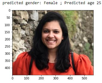
With the above, we can see that we are able to make predictions for both age and gender in a single shot. However, we need to note that this is highly unstable and that the age value varies considerably with different orientations of the image and also lighting conditions. Data augmentation comes in handy in such a scenario.

So far, we have learned about transfer learning, pre-trained architectures, and how to leverage them in two different use cases. You would have also noticed that the code is slightly on the lengthier side where we import extensive packages manually, create empty lists to log metrics, and constantly read/show images for debugging purposes. In the next section, we will learn about a library that the authors have built to avoid such verbose code.

Introducing the torch_snippets library

As you may have noticed, we are using the same functions in almost all the sections. It is a waste of our time to write the same lines of functions again and again. For convenience, the authors of this book have written a Python library by the name of torch_snippets so that our code looks short and clean.

Utilities such as reading an image, showing an image, and the entire training loop are quite repetitive. We want to circumvent writing the same functions over and over by wrapping them in code that is preferably a single function call. For example, to read a color image, we need not write cv2.imread(...) followed by cv2.cvtColor(...) every time. Instead, we can simply call read(...). Similarly, for plt.imshow(...), there are numerous hassles, including the fact that the size of the image should be optimal, and that the channel dimension should be last (remember PyTorch has them first). These will always be taken care of by the single function, show. Similar to read and show, there are over 20 convenience functions and classes that we will be using throughout the book. We will use torch_snippets from now on so as to focus more on actual deep learning without distractions. Let's dive a little and understand the salient functions by training age-and-gender with this library instead so that we can learn to use these functions and derive the maximum benefit.

1. Install and load the library:

!pip install torch_snippets
from torch_snippets import *

Right out of the gate, the library allows us to load all the important torch modules and utilities such as NumPy, pandas, Matplotlib, Glob, Os, and more.

2. Download the data and create a dataset as in the previous section. Create a dataset class, GenderAgeClass, with a few changes, which are shown in bold in the following code:

class GenderAgeClass(Dataset):
    ...
    def __getitem__(self, ix):
        ...
        age = f.age
        im = read(file, 1)
        return im, age, gen

    def preprocess_image(self, im):
        im = resize(im, IMAGE_SIZE)
        im = torch.tensor(im).permute(2,0,1)
        ...

In the preceding code block, the line im = read(file, 1) is wrapping cv2.imread and cv2.COLOR_BGR2RGB into a single function call. The "1" stands for "read as color image", and if not given, will load a black and white image by default. There is also a resize function that wraps cv2.resize. Next, let's look at the show function.

3. Specify the training and validation datasets and view the sample images:

trn = GenderAgeClass(trn_df)
val = GenderAgeClass(val_df)
train_loader = DataLoader(trn, batch_size=32, shuffle=True, 
                  drop_last=True, collate_fn=trn.collate_fn)
test_loader = DataLoader(val, batch_size=32, 
                         collate_fn=val.collate_fn)

im, gen, age = trn[0]
show(im, title=f'Gender: {gen}
Age: {age}', sz=5)

As we are dealing with images throughout the book, it makes sense to wrap import matplotlib.pyplot as plt and plt.imshow into a function. Calling show(<2D/3D-Tensor>) will do exactly that. Unlike Matplotlib, it can plot torch arrays present on the GPU, irrespective of whether the image contains a channel as the first dimension or the last dimension. The keyword title will plot a title with the image, and the keyword sz (short for size) will plot a larger/smaller image based on the integer value passed (if not passed, sz will pick a sensible default based on image resolution). During object detection chapters, we will use the same function to show bounding boxes as well. Check out help(show) for more arguments. Let's create some datasets here and inspect the first batch of images along with their targets.

4. Create data loaders and inspect the tensors. Inspecting tensors for their data type, min, mean, max, and shape is such a common activity that it is wrapped as a function. It can accept any number of tensor inputs:

train_loader = DataLoader(trn, batch_size=32, shuffle=True, 
                drop_last=True, collate_fn=trn.collate_fn)
test_loader = DataLoader(val, batch_size=32, 
                         collate_fn=val.collate_fn)

ims, gens, ages = next(iter(train_loader))
inspect(ims, gens, ages)

The inspect output will look like this:

============================================================
Tensor Shape: torch.Size([32, 3, 224, 224]) Min: -2.118 Max: 2.640 Mean: 0.133 dtype: torch.float32
============================================================
Tensor Shape: torch.Size([32]) Min: 0.000 Max: 1.000 Mean: 0.594 dtype: torch.float32 
============================================================
Tensor Shape: torch.Size([32]) Min: 0.087 Max: 0.925 Mean: 0.400 dtype: torch.float32 
============================================================

5. Create model, optimizer, loss_functions, train_batch, and validate_batch as usual. As each deep learning experiment is unique, there aren't any wrapper functions for this step.

6. Finally, we need to load all the components and start training. Log the metrics over increasing epochs.

This is a highly repetitive loop with minimal changes required. We will always loop over a fixed number of epochs, first over the train data loader, and then over the validation data loader. Each batch is called using either train_batch or validate_batch, every time that you have to create empty lists of metrics and keep track of them after training/ validation. At the end of an epoch, you have to print the averages of all of these metrics and repeat the task. It is also helpful that you know how long (in seconds) each epoch /batch is going to train for. Finally, at the end of the training, it is common to plot the same metrics using matplotlib. All of these are wrapped into a single utility called Report. It is a Python class that has different methods to understand. The bold parts in the following code highlight the functionality of Report:

model, criterion, optimizer = get_model()
n_epochs = 5
log = Report(n_epochs)
for epoch in range(n_epochs):
    N = len(train_loader)
    for ix, data in enumerate(train_loader):
        total_loss,gender_loss,age_loss = train_batch(data, 
                                  model, optimizer, criterion)
        log.record(epoch+(ix+1)/N, trn_loss=total_loss, 
                                                end='
')

    N = len(test_loader)
    for ix, data in enumerate(test_loader):
        total_loss,gender_acc,age_mae = validate_batch(data, 
                                             model, criterion)
        gender_acc /= len(data[0])
        age_mae /= len(data[0])
        log.record(epoch+(ix+1)/N, val_loss=total_loss, 
                   val_gender_acc=gender_acc, 
                   val_age_mae=age_mae, end='
')
    log.report_avgs(epoch+1)
log.plot_epochs()

The Report class is instantiated with the only argument, the number of epochs to be trained on, and is instantiated just before the start of training.

At each train/validation step, we can call the Report.record method with exactly one positional argument, which is the position (in terms of batch number) of training/ validation we are at (typically, this is ( epoch_number + (1+batch number)/(total_N_batches) ). Following the positional argument, we pass a bunch of keyword arguments that we are free to choose. If it's training loss that needs to be captured, the keyword argument could be trn_loss. In the preceding, we are logging four metrics, trn_loss, val_loss, val_gender_acc, and val_age_mae, without creating a single empty list.

Not only does it record, but it will also print the same losses in the output. The use of ' ' as an end argument is a special way of saying replace this line the next time a new set of losses are to be recorded. Furthermore, Report will compute the time remaining for training and validation automatically and print that too.

Report will remember when the metric was logged and print all the average metrics at that epoch when the Report.report_avgs function is called. This will be a permanent print.

Finally, the same average metrics are plotted as a line chart in the function call Report.plot_epochs, without the need for formatting (you can also use Report.plot for plotting every batch metric of the entire training, but this might look messy). The same function can selectively plot metrics if asked for. By way of an example, in the preceding case, if you are interested in plotting only the trn_loss and val_loss metrics, this can be done by calling log.plot_epochs(['trn_loss, 'val_loss']) or even simply log.plot_epochs('_loss'). It will search for a string match with all the metrics and figure out what metrics we are asking for.

Once training is complete, the output for the preceding code snippet should look like this:

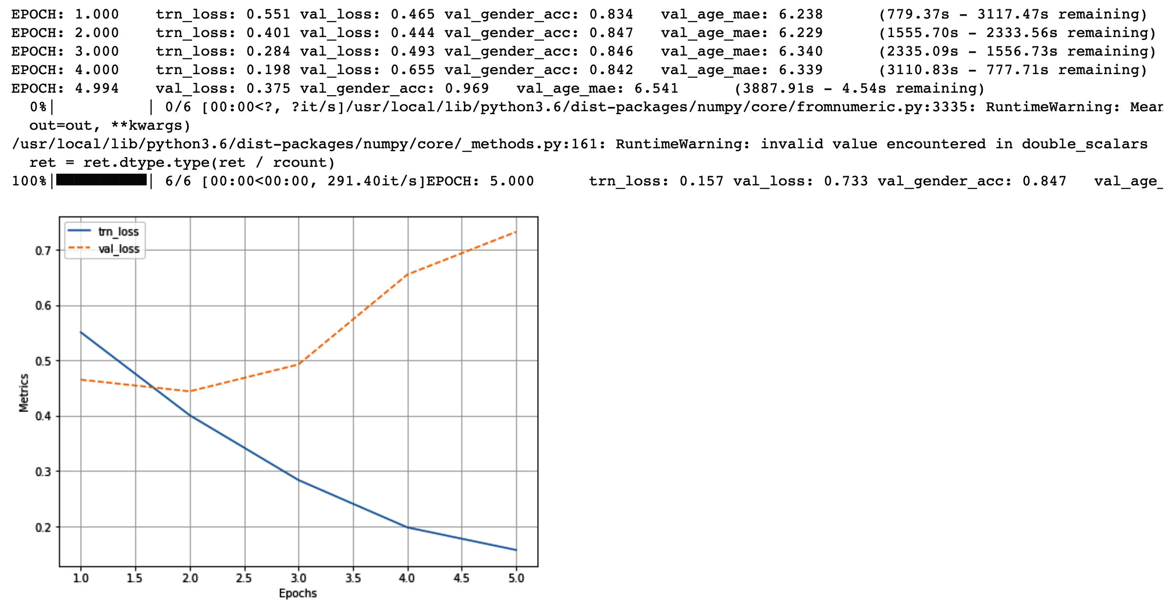
7. Load a sample image and effect a prediction:

!wget -q https://www.dropbox.com/s/6kzr8l68e9kpjkf/5_9.JPG
IM = read('/content/5_9.JPG', 1)
im = trn.preprocess_image(IM).to(device)

gender, age = model(im)
pred_gender = gender.to('cpu').detach().numpy()
pred_age = age.to('cpu').detach().numpy()

info = f'predicted gender: {np.where(pred_gender[0][0]<0.5, 
"Male","Female")}
 Predicted age {int(pred_age[0][0]*80)}'
show(IM, title=info, sz=10)

To summarize, here are the important functions (and the functions they are wrapped around) that we will use in the rest of the book wherever needed:

• from torch_snippets import *
• Glob (glob.glob)
• Choose (np.random.choice)
• Read (cv2.imread)
• Show (plt.imshow)
• Subplots (plt.subplots – show a list of images)
• Inspect (tensor.min, tensor.mean, tensor.max, tensor.shape, and tensor.dtype – statistics of several tensors)
• Report (keeping track of all metrics while training and plotting them after training)

You can view the complete list of functions by running torch_snippets; print(dir(torch_snippets)). For each function, you can print its help using help(function) or even simply ??function in a Jupyter notebook. With the understanding of leveraging torch_snippets, you should be able to simplify code considerably. You will notice this in action starting with the next chapter.

Summary

In this chapter, we have learned about how transfer learning helps to achieve high accuracy, even with a smaller number of data points. We have also learned about the popular pre-trained models, VGG and ResNet. Furthermore, we understood how to build models when we are trying to predict different scenarios, such as the location of key points on a face and combining loss values while training a model to predict for both age and gender together, where age is of a certain data type and gender is of a different data type.

With this foundation of image classification through transfer learning, in the next chapter, we will learn about some of the practical aspects of training an image classification model. We will learn about how to explain a model and also learn the tricks of how to train a model to achieve high accuracy and finally, learn the pitfalls that a practitioner needs to avoid while implementing a trained model.

Questions

1. What are VGG and ResNet pre-trained architectures trained on?
2. Why does VGG11 have an inferior accuracy to VGG16?
3. What does the number 11 in VGG11 represent?
4. What is residual in the residual network?
5. What is the advantage of a residual network?
6. What are the various popular pre-trained models?
7. During transfer learning, why should images be normalized with the same mean and standard deviation as those that were used during the training of a pre-trained model?
8. Why do we freeze certain parameters in a model?
9. How do we know the various modules that are present in a pre-trained model?
10. How do we train a model that predicts categorical and numerical values together?
11. Why might age and gender prediction code not always work for an image of your own interest if we execute the same code as we wrote in the age and gender estimation section?
12. How can we further improve the accuracy of the facial keypoint recognition model that we wrote about in the facial key points prediction section?