
In previous chapters, we learned about leveraging convolutional neural networks (CNNs) along with pre-trained models to perform image classification. This chapter will further solidify our understanding of CNNs and the various practical aspects to be considered when leveraging them in real-world applications. We will start by understanding the reasons why CNNs predict the classes that they do by using class activation maps (CAMs). Following this, we will understand the various data augmentations that can be done to improve the accuracy of a model. Finally, we will learn about the various instances where models could go wrong in the real world and highlight the aspects that should be taken care of in such scenarios to avoid pitfalls.
The following topics will be covered in this chapter:
- Generating CAMs
- Understanding the impact of batch normalization and data augmentation
- Practical aspects to take care of during model implementation
Generating CAMs
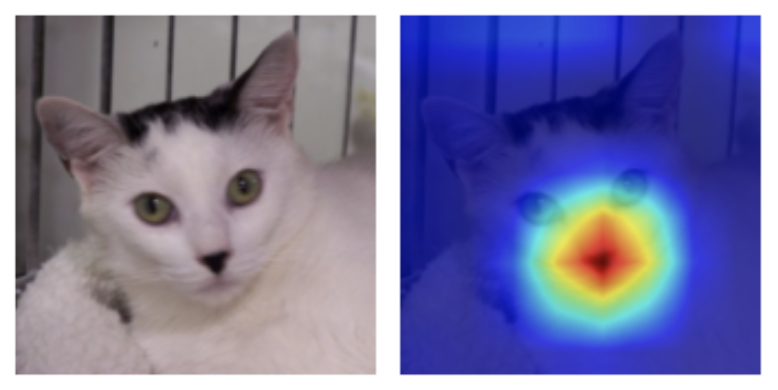
Imagine a scenario where you have built a model that is able to make good predictions. However, the stakeholder that you are presenting the model to wants to understand the reason why the model predictions are as they are. CAMs come in handy in this scenario. An example CAM is as follows, where we have the input image on the left and the pixels that were used to come up with the class prediction highlighted on the right:
Let's understand how CAMs can be generated once a model is trained. Feature maps are intermediate activations that come after a convolution operation. Typically, the shape of these activation maps is n-channels x height x width. If we take the mean of all these activations, they show the hotspots of all the classes in the image. But if we are interested in locations that are only important for a particular class (say, cat), we need to figure out only those feature maps among n-channels that are responsible for that class. For the convolution layer that generated these feature maps, we can compute its gradients with respect to the cat class. Note that only those channels that are responsible for predicting cat will have a high gradient. This means that we can use the gradient information to give weightage to each of n-channels and obtain an activation map exclusively for cat.
Now that we understand the high-level strategy of how to generate CAMs, let's put it into practice step by step:
- Decide for which class you want to calculate the CAM and for which convolutional layer in the neural network you want to compute the CAM.
- Calculate the activations arising from any convolutional layer – let's say the feature shape at a random convolution layer is 512 x 7 x 7.
- Fetch the gradient values arising from this layer with respect to the class of interest. The output gradient shape is 256 x 512 x 3 x 3 (which is the shape of the convolutional tensor – that is, in-channels x out-channels x kernel-size x kernel-size).
- Compute the mean of the gradients within each output channel. The output shape is 512.
- Calculate the weighted activation map – which is the multiplication of the 512 gradient means by the 512 activation channels. The output shape is 512 x 7 x 7.
- Compute the mean (across 512 channels) of the weighted activation map to fetch an output of the shape 7 x 7.
- Resize (upscale) the weighted activation map outputs to fetch an image of a size that is of the same size as the input. This is done so that we have an activation map that resembles the original image.
- Overlay the weighted activation map onto the input image.
The following diagram from the paper Grad-CAM: Gradient-weighted Class Activation Mapping (https://arxiv.org/abs/1610.02391) pictorially describes the preceding steps:

The key to the entire process lies in step 5. We consider two aspects of the step:
- If a certain pixel is important, then the CNN will have a large activation at those pixels.
- If a certain convolutional channel is important with respect to the required class, the gradients at that channel will be very large.
On multiplying these two, we indeed end up with a map of importance across all the pixels.
The preceding strategy is implemented in code to understand the reason why the CNN model predicts that an image indicates the likelihood of an incident of malaria, as follows:
- Download the dataset and import the relevant packages:
import os
if not os.path.exists('cell_images'):
    !pip install -U -q torch_snippets
    !wget -q ftp://lhcftp.nlm.nih.gov/Open-Access-Datasets/
     Malaria/cell_images.zip
    !unzip -qq cell_images.zip
    !rm cell_images.zip
from torch_snippets import *
- Specify the indices corresponding to the output classes:
id2int = {'Parasitized': 0, 'Uninfected': 1}
- Perform the transformations to be done on top of the images:
from torchvision import transforms as T

trn_tfms = T.Compose([
                T.ToPILImage(),
                T.Resize(128),
                T.CenterCrop(128),
                T.ColorJitter(brightness=(0.95,1.05),
                              contrast=(0.95,1.05),
                              saturation=(0.95,1.05),
                              hue=0.05),
                T.RandomAffine(5, translate=(0.01,0.1)),
                T.ToTensor(),
                T.Normalize(mean=[0.5, 0.5, 0.5],
                            std=[0.5, 0.5, 0.5]),
            ])
In the preceding code, we have a pipeline of transformations on top of the input image – which is a pipeline of resizing the image (which ensures that the minimum size of one of the dimensions is 128, in this case) and then cropping it from the center. Furthermore, we are performing random color jittering and affine transformation. Next, we are scaling an image using the .ToTensor method to have a value between 0 and 1, and finally, we are normalizing the image. As discussed in Chapter 4, Introducing Convolutional Neural Networks, we can also use the imgaug library.
- Specify the transformations to be done on the validation images:
val_tfms = T.Compose([
                T.ToPILImage(),
                T.Resize(128),
                T.CenterCrop(128),
                T.ToTensor(),
                T.Normalize(mean=[0.5, 0.5, 0.5],
                            std=[0.5, 0.5, 0.5]),
            ])
- Define the dataset class – MalariaImages:
class MalariaImages(Dataset):

    def __init__(self, files, transform=None):
        self.files = files
        self.transform = transform
        logger.info(len(self))

    def __len__(self):
        return len(self.files)

    def __getitem__(self, ix):
        fpath = self.files[ix]
        clss = fname(parent(fpath))
        img = read(fpath, 1)
        return img, clss

    def choose(self):
        return self[randint(len(self))]

    def collate_fn(self, batch):
        _imgs, classes = list(zip(*batch))
        if self.transform:
            imgs = [self.transform(img)[None]
                    for img in _imgs]
        classes = [torch.tensor([id2int[clss]])
                   for class in classes]
        imgs, classes = [torch.cat(i).to(device)
                         for i in [imgs, classes]]
        return imgs, classes, _imgs
- Fetch the training and validation datasets and dataloaders:
device = 'cuda' if torch.cuda.is_available() else 'cpu'
all_files = Glob('cell_images/*/*.png')
np.random.seed(10)
np.random.shuffle(all_files)

from sklearn.model_selection import train_test_split
trn_files, val_files = train_test_split(all_files,
                                        random_state=1)

trn_ds = MalariaImages(trn_files, transform=trn_tfms)
val_ds = MalariaImages(val_files, transform=val_tfms)
trn_dl = DataLoader(trn_ds, 32, shuffle=True,
                    collate_fn=trn_ds.collate_fn)
val_dl = DataLoader(val_ds, 32, shuffle=False,
                    collate_fn=val_ds.collate_fn)
- Define the model – MalariaClassifier:
def convBlock(ni, no):
    return nn.Sequential(
        nn.Dropout(0.2),
        nn.Conv2d(ni, no, kernel_size=3, padding=1),
        nn.ReLU(inplace=True),
        nn.BatchNorm2d(no),
        nn.MaxPool2d(2),
    )

class MalariaClassifier(nn.Module):
    def __init__(self):
        super().__init__()
        self.model = nn.Sequential(
            convBlock(3, 64),
            convBlock(64, 64),
            convBlock(64, 128),
            convBlock(128, 256),
            convBlock(256, 512),
            convBlock(512, 64),
            nn.Flatten(),
            nn.Linear(256, 256),
            nn.Dropout(0.2),
            nn.ReLU(inplace=True),
            nn.Linear(256, len(id2int))
        )
        self.loss_fn = nn.CrossEntropyLoss()

    def forward(self, x):
        return self.model(x)

    def compute_metrics(self, preds, targets):
        loss = self.loss_fn(preds, targets)
        acc =(torch.max(preds, 1)[1]==targets).float().mean()
        return loss, acc
- Define the functions to train and validate on a batch of data:
def train_batch(model, data, optimizer, criterion):
    model.train()
    ims, labels, _ = data
    _preds = model(ims)
    optimizer.zero_grad()
    loss, acc = criterion(_preds, labels)
    loss.backward()
    optimizer.step()
    return loss.item(), acc.item()

@torch.no_grad()
def validate_batch(model, data, criterion):
    model.eval()
    ims, labels, _ = data
    _preds = model(ims)
    loss, acc = criterion(_preds, labels)
    return loss.item(), acc.item()
- Train the model over increasing epochs:
model = MalariaClassifier().to(device)
criterion = model.compute_metrics
optimizer = optim.Adam(model.parameters(), lr=1e-3)
n_epochs = 2

log = Report(n_epochs)
for ex in range(n_epochs):
    N = len(trn_dl)
    for bx, data in enumerate(trn_dl):
        loss, acc = train_batch(model, data, optimizer,
                                    criterion)
        log.record(ex+(bx+1)/N,trn_loss=loss,trn_acc=acc,
                                    end='
')

    N = len(val_dl)
    for bx, data in enumerate(val_dl):
        loss, acc = validate_batch(model, data, criterion)
        log.record(ex+(bx+1)/N,val_loss=loss,val_acc=acc,
                                    end='
')

    log.report_avgs(ex+1)
- Fetch the convolution layer in the fifth convBlock in the model:
im2fmap = nn.Sequential(*(list(model.model[:5].children())+
                        list(model.model[5][:2].children())))
In the preceding line of code, we are fetching the fourth layer of the model and also the first two layers within convBlock – which happens to be the Conv2D layer.
- Define the im2gradCAM function that takes an input image and fetches the heatmap corresponding to activations of the image:
def im2gradCAM(x):
    model.eval()
    logits = model(x)
    heatmaps = []
    activations = im2fmap(x)
    print(activations.shape)
    pred = logits.max(-1)[-1]
    # get the model's prediction
    model.zero_grad()
    # compute gradients with respect to
    # model's most confident logit
    logits[0,pred].backward(retain_graph=True)
    # get the gradients at the required featuremap location
    # and take the avg gradient for every featuremap
    pooled_grads = model.model[-7][1]
                        .weight.grad.data.mean((0,2,3))
    # multiply each activation map with
    # corresponding gradient average
    for i in range(activations.shape[1]):
        activations[:,i,:,:] *= pooled_grads[i]
    # take the mean of all weighted activation maps
    # (that has been weighted by avg. grad at each fmap)
    heatmap =torch.mean(activations, dim=1)[0].cpu().detach()
    return heatmap, 'Uninfected' if pred.item()
else 'Parasitized'
- Define the upsampleHeatmap function to up-sample the heatmap to a shape that corresponds to the shape of the image:
SZ = 128
def upsampleHeatmap(map, img):
    m,M = map.min(), map.max()
    map = 255 * ((map-m) / (M-m))
    map = np.uint8(map)
    map = cv2.resize(map, (SZ,SZ))
    map = cv2.applyColorMap(255-map, cv2.COLORMAP_JET)
    map = np.uint8(map)
    map = np.uint8(map*0.7 + img*0.3)
    return map
In the preceding lines of code, we are de-normalizing the image and also overlaying the heatmap on top of the image.
- Run the preceding functions on a set of images:
N = 20
_val_dl = DataLoader(val_ds, batch_size=N, shuffle=True,
                     collate_fn=val_ds.collate_fn)
x,y,z = next(iter(_val_dl))

for i in range(N):
    image = resize(z[i], SZ)
    heatmap, pred = im2gradCAM(x[i:i+1])
    if(pred=='Uninfected'):
        continue
    heatmap = upsampleHeatmap(heatmap, image)
    subplots([image, heatmap], nc=2, figsize=(5,3),
                suptitle=pred)
The output of the preceding code is as follows:
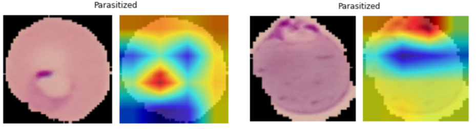
From this, we can see that the prediction is as it is because of the content that is highlighted in red (which has the highest CAM value).
Now that we have learned about generating class activation heatmaps for images using a trained model, we are in a position to explain what makes a certain classification so.
In the next section, let's learn about additional tricks around data augmentation that can help when building models.
Understanding the impact of data augmentation and batch normalization
One clever way of improving the accuracy of models is by leveraging data augmentation. We have already seen this in Chapter 4, Introducing Convolutional Neural Networks, where we used data augmentation to improve the accuracy of classification on a translated image. In the real world, you would encounter images that have different properties – for example, some images might be much brighter, some might contain objects of interest near the edges, and some images might be more jittery than others. In this section, we will learn about how the usage of data augmentation can help in improving the accuracy of a model. Furthermore, we will learn about how data augmentation can practically be a pseudo-regularizer for our models.
To understand the impact of data augmentation and batch normalization, we will go through a dataset of recognizing traffic signs. We will evaluate three scenarios:
- No batch normalization/data augmentation
- Only batch normalization, but no data augmentation
- Both batch normalization and data augmentation
Note that given that the dataset and processing remain the same across the three scenarios, and only the data augmentation and model (the addition of the batch normalization layer) differ, we will only provide the following code for the first scenario, but the other two scenarios are available in the notebook on GitHub.
Coding up road sign detection
Let's code up for road sign detection without data augmentation and batch normalization, as follows:
- Download the dataset and import the relevant packages:
import os
if not os.path.exists('GTSRB'):
    !pip install -U -q torch_snippets
    !wget -qq https://sid.erda.dk/public/archives/
        daaeac0d7ce1152aea9b61d9f1e19370/
        GTSRB_Final_Training_Images.zip
    !wget -qq https://sid.erda.dk/public/archives/
        daaeac0d7ce1152aea9b61d9f1e19370/
        GTSRB_Final_Test_Images.zip
    !unzip -qq GTSRB_Final_Training_Images.zip
    !unzip -qq GTSRB_Final_Test_Images.zip
    !wget https://raw.githubusercontent.com/georgesung/
     traffic_sign_classification_german/master/signnames.csv
    !rm GTSRB_Final_Training_Images.zip
       GTSRB_Final_Test_Images.zip

from torch_snippets import *
- Assign the class IDs to possible output classes:
classIds = pd.read_csv('signnames.csv')
classIds.set_index('ClassId', inplace=True)
classIds = classIds.to_dict()['SignName']
classIds = {f'{k:05d}':v for k,v in classIds.items()}
id2int = {v:ix for ix,(k,v) in enumerate(classIds.items())}
- Define the transformation pipeline on top of the images without any augmentation:
from torchvision import transforms as T
trn_tfms = T.Compose([
                T.ToPILImage(),
                T.Resize(32),
                T.CenterCrop(32),
                # T.ColorJitter(brightness=(0.8,1.2),
                # contrast=(0.8,1.2),
                # saturation=(0.8,1.2),
                # hue=0.25),
                # T.RandomAffine(5, translate=(0.01,0.1)),
                T.ToTensor(),
                T.Normalize(mean=[0.485, 0.456, 0.406],
                            std=[0.229, 0.224, 0.225]),
            ])
val_tfms = T.Compose([
                T.ToPILImage(),
                T.Resize(32),
                T.CenterCrop(32),
                T.ToTensor(),
                T.Normalize(mean=[0.485, 0.456, 0.406],
                            std=[0.229, 0.224, 0.225]),
            ])
In the preceding code, we are specifying that we convert each image into a PIL image and resize and crop the image from the center. Furthermore, we are scaling the image to have pixel values that are between 0 and 1 using the .ToTensor method. Finally, we are normalizing the input image so that a pre-trained model can be leveraged.
- Define the dataset class – GTSRB:
class GTSRB(Dataset):

    def __init__(self, files, transform=None):
        self.files = files
        self.transform = transform
        logger.info(len(self))

    def __len__(self):
        return len(self.files)

    def __getitem__(self, ix):
        fpath = self.files[ix]
        clss = fname(parent(fpath))
        img = read(fpath, 1)
        return img, classIds[clss]

    def choose(self):
        return self[randint(len(self))]
    def collate_fn(self, batch):
        imgs, classes = list(zip(*batch))
        if self.transform:
            imgs =[self.transform(img)[None]
                   for img in imgs]
        classes = [torch.tensor([id2int[clss]])
                   for clss in classes]
        imgs, classes = [torch.cat(i).to(device)
                         for i in [imgs, classes]]
        return imgs, classes
- Create the training and validation datasets and dataloaders:
device = 'cuda' if torch.cuda.is_available() else 'cpu'
all_files = Glob('GTSRB/Final_Training/Images/*/*.ppm')
np.random.seed(10)
np.random.shuffle(all_files)

from sklearn.model_selection import train_test_split
trn_files, val_files = train_test_split(all_files,
                                        random_state=1)

trn_ds = GTSRB(trn_files, transform=trn_tfms)
val_ds = GTSRB(val_files, transform=val_tfms)
trn_dl = DataLoader(trn_ds, 32, shuffle=True,
                    collate_fn=trn_ds.collate_fn)
val_dl = DataLoader(val_ds, 32, shuffle=False,
                    collate_fn=val_ds.collate_fn)
- Define the model – SignClassifier:
import torchvision.models as models

def convBlock(ni, no):
    return nn.Sequential(
                nn.Dropout(0.2),
                nn.Conv2d(ni, no, kernel_size=3, padding=1),
                nn.ReLU(inplace=True),
                #nn.BatchNorm2d(no),
                nn.MaxPool2d(2),
            )

class SignClassifier(nn.Module):
    def __init__(self):
        super().__init__()
        self.model = nn.Sequential(
                        convBlock(3, 64),
                        convBlock(64, 64),
                        convBlock(64, 128),
                        convBlock(128, 64),
                        nn.Flatten(),
                        nn.Linear(256, 256),
                        nn.Dropout(0.2),
                        nn.ReLU(inplace=True),
                        nn.Linear(256, len(id2int))
                    )
        self.loss_fn = nn.CrossEntropyLoss()

    def forward(self, x):
        return self.model(x)

    def compute_metrics(self, preds, targets):
        ce_loss = self.loss_fn(preds, targets)
        acc =(torch.max(preds, 1)[1]==targets).float().mean()
        return ce_loss, acc
- Define the functions to train and validate on a batch of data, respectively:
def train_batch(model, data, optimizer, criterion):
    model.train()
    ims, labels = data
    _preds = model(ims)
    optimizer.zero_grad()
    loss, acc = criterion(_preds, labels)
    loss.backward()
    optimizer.step()
    return loss.item(), acc.item()

@torch.no_grad()
def validate_batch(model, data, criterion):
    model.eval()
    ims, labels = data
    _preds = model(ims)
    loss, acc = criterion(_preds, labels)
    return loss.item(), acc.item()
- Define the model and train it over increasing epochs:
model = SignClassifier().to(device)
criterion = model.compute_metrics
optimizer = optim.Adam(model.parameters(), lr=1e-3)
n_epochs = 50

log = Report(n_epochs)
for ex in range(n_epochs):
    N = len(trn_dl)
    for bx, data in enumerate(trn_dl):
        loss, acc = train_batch(model, data, optimizer,
                                    criterion)
        log.record(ex+(bx+1)/N,trn_loss=loss, trn_acc=acc,
                                     end='
')

    N = len(val_dl)
    for bx, data in enumerate(val_dl):
        loss, acc = validate_batch(model, data, criterion)
        log.record(ex+(bx+1)/N, val_loss=loss, val_acc=acc,
                                    end='
')

    log.report_avgs(ex+1)
    if ex == 10: optimizer = optim.Adam(model.parameters(),
                                    lr=1e-4)
The lines of code that are bold are the ones that you would change in the three scenarios. The results of the three scenarios in terms of training and validation accuracy are as follows:
| Augment | Batch-Norm | Train Accuracy | Validation Accuracy |
| No | No | 95.9 | 94.5 |
| No | Yes | 99.3 | 97.7 |
| Yes | Yes | 97.7 | 97.6 |
Note that in the preceding three scenarios, we see the following:
- The model did not have as high accuracy when there was no batch normalization.
- The accuracy of the model increased considerably but also the model overfitted on training data when we had batch normalization only but no data augmentation.
- The model with both batch normalization and data augmentation had high accuracy and minimal overfitting (as the training and validation loss values are very similar).
With the importance of batch normalization and data augmentation in place, in the next section, we will learn about some key aspects to take care of when training/implementing our image classification models.
Practical aspects to take care of during model implementation
So far, we have seen the various ways of building an image classification model. In this section, we will learn about some of the practical considerations that need to be taken care of when building models. The ones we will discuss in this chapter are as follows:
- Dealing with imbalanced data
- The size of an object within an image when performing classification
- The difference between training and validation images
- The number of convolutional and pooling layers in a network
- Image sizes to train on GPUs
- Leveraging OpenCV utilities
Dealing with imbalanced data
Imagine a scenario where you are trying to predict an object that occurs very rarely within our dataset – let's say in 1% of the total images. For example, this can be the task of predicting whether an X-ray image suggests a rare lung infection.
How do we measure the accuracy of the model that is trained to predict the rare lung infection? If we simply predict a class of no infection for all images, the accuracy of classification is 99%, while still being useless. A confusion matrix that depicts the number of times the rare object class has occurred and the number of times the model predicted the rare object class correctly comes in handy in this scenario. Thus, the right set of metrics to look at in this scenario is the metrics related to the confusion matrix.
A typical confusion matrix looks as follows:

In the preceding confusion matrix, 0 stands for no infection and 1 stands for infection. Typically, we would fill up the matrix to understand how accurate our model is.
Next comes the question of ensuring that the model gets trained. Typically, the loss function (binary or categorical cross-entropy) takes care of ensuring that the loss values are high when the amount of misclassification is high. However, in addition to the loss function, we can also assign a higher weight to the rarely occurring class, thereby ensuring that we explicitly mention to the model that we want to correctly classify the rare class images.
In addition to assigning class weights, we have already seen that image augmentation and/or transfer learning help considerably in improving the accuracy of the model. Furthermore, when augmenting an image, we can over-sample the rare class images to increase their mix in the overall population.
The size of the object within an image
Imagine a scenario where the presence of a small patch within a large image dictates the class of the image – for example, lung infection identification where the presence of certain tiny nodules indicates an incident of the disease. In such a scenario, image classification is likely to result in inaccurate results, as the object occupies a smaller portion of the entire image. Object detection comes in handy in this scenario (which we will study in the next chapter).
A high-level intuition to solve these problems would be to first divide the input images into smaller grid cells (let's say a 10 x 10 grid) and then identify whether a grid cell contains the object of interest.
Dealing with the difference between training and validation data
Imagine a scenario where you have built a model to predict whether the image of an eye indicates that the person is likely to be suffering from diabetic retinopathy. To build the model, you have collected data, curated it, cropped it, normalized it, and then finally built a model that has very high accuracy on validation images. However, hypothetically, when the model is used in a real setting (let's say by a doctor/nurse), the model is not able to predict well. Let's understand a few possible reasons why:
- Are the images taken at the doctor's office similar to the images used to train the model?
- Images used when training and real-world images could be very different if you built a model on a curated set of data that has all the preprocessing done, while the images taken at the doctor's end are non-curated.
- Images could be different if the device used to capture images at the doctor's office has a different resolution of capturing images when compared to the device used to collect images that are used for training.
- Images can be different if there are different lighting conditions at which the images are getting captured in both places.
- Are the subjects (images) representative enough of the overall population?
- Images are representative if they are trained on images of the male population but are tested on the female population, or if, in general, the training and real-world images correspond to different demographics.
- Is the training and validation split done methodically?
- Imagine a scenario where there are 10,000 images and the first 5,000 images belong to one class and the last 5,000 images belong to another class. When building a model, if we do not randomize but split the dataset into training and validation with consecutive indices (without random indices), we are likely to see a higher representation of one class while training and of the other class during validation.
In general, we need to ensure that the training, validation, and real-world images all have similar data distribution before an end user leverages the system.
The number of nodes in the flatten layer
Consider a scenario where you are working on images that are 300 x 300 in dimensions. Technically, we can perform more than five convolutional pooling operations to get the final layer that has as many features as possible. Furthermore, we can have as many channels as we want in this scenario within a CNN. Practically, though, in general, we would design a network so that it has 500–5,000 nodes in the flatten layer.
As we saw in Chapter 4, Introducing Convolutional Neural Networks, if we have a greater number of nodes in the flatten layer, we would have a very high number of parameters when the flatten layer is connected to the subsequent dense layer before connecting to the final classification layer.
In general, it is good practice to have a pre-trained model that obtains the flatten layer so that relevant filters are activated as appropriate. Furthermore, when leveraging pre-trained models, make sure to freeze the parameters of the pre-trained model.
Generally, the number of trainable parameters in a CNN can be anywhere between 1 million to 10 million in a less complex classification exercise.
Image size
Let's say we are working on images that are of very high dimensions – for example, 2,000 x 1,000 in shape. When working on such large images, we need to consider the following possibilities:
- Can the images be resized to lower dimensions? Images of objects might not lose information if resized; however, images of text documents might lose considerable information if resized to a smaller size.
- Can we have a lower batch size so that the batch fits into GPU memory? Typically, if we are working with large images, there is a good chance that for the given batch size, the GPU memory is not sufficient to perform computations on the batch of images.
- Do certain portions of the image contain the majority of the information, and hence can the rest of the image be cropped?
Leveraging OpenCV utilities
OpenCV is an open source package that has extensive modules that help in fetching information from images (more on OpenCV utilities in Chapter 18, Using OpenCV Utilities for Image Analysis). It was one of the most prominent libraries used prior to the deep learning revolution in computer vision. Traditionally, it has been built on top of multiple hand-engineered features and at the time of writing this book, OpenCV has a few packages that integrate deep learning models' outputs.
Imagine a scenario where you have to move a model to production; less complexity is generally preferable in such a scenario – sometimes even at the cost of accuracy. If any OpenCV module solves the problem that you are already trying to solve, in general, it should be preferred over building a model (unless building a model from scratch gives a considerable boost in accuracy than leveraging off-the-shelf modules).
Summary
In this chapter, we learned about multiple practical aspects that we need to take into consideration when building CNN models – batch normalization, data augmentation, explaining the outcomes using CAMs, and some scenarios that you need to be aware of when moving a model to production.
In the next chapter, we will switch gears and learn about the fundamentals of object detection – where we will not only identify the classes corresponding to objects in an image but also draw a bounding box around the location of the object.
Questions
- How are CAMs obtained?
- How do batch normalization and data augmentation help when training a model?
- What are the common reasons why a CNN model overfits?
- What are the various scenarios where the CNN model works with training and validation data at the data scientists' end but not in the real world?
- What are the various scenarios where we leverage OpenCV packages?