In the previous chapter, we learned about the fundamental building blocks of a neural network and also implemented forward and back-propagation from scratch in Python.

In this chapter, we will dive into the foundations of building a neural network using PyTorch, which we will leverage multiple times in subsequent chapters when we learn about various use cases in image analysis. We will start by learning about the core data type that PyTorch works on – tensor objects. We will then dive deep into the various operations that can be performed on tensor objects and how to leverage them when building a neural network model on top of a toy dataset (so that we strengthen our understanding before we gradually look at more realistic datasets, starting with the next chapter). This will allow us so to gain an intuition of how to build neural network models using PyTorch to map input and output values. Finally, we will learn about implementing custom loss functions so that we can customize based on the use case we are solving.

Specifically, this chapter will cover the following topics:

• Installing PyTorch
• PyTorch tensors
• Building a neural network using PyTorch
• Using a sequential method to build a neural network
• Saving and loading a PyTorch model

Installing PyTorch

PyTorch provides multiple functionalities that aid in building a neural network – abstracting the various components using high-level methods and also providing us with tensor objects that leverage GPUs to train a neural network faster.

Before installing PyTorch, we first need to install Python, as follows:

1. To install Python, we'll use the anaconda.com/distribution/ platform to fetch an installer that will install Python as well as important deep learning-specific libraries for us automatically:

Choose the graphical installer of the latest Python version 3.xx (3.7, as of the time of writing this book) and let it download.

2. Install it using the downloaded installer:

Next, we'll install PyTorch, which is equally simple.

3. Visit the QUICK START LOCALLY section on the https://pytorch.org/ website and choose your operating system (Your OS), Conda for Package, Python for Language, and None for CUDA. If you have CUDA libraries, you may choose the appropriate version:

This will prompt you to run a command such as conda install pytorch torchvision cpuonly -c pytorch in your terminal.

4. Run the command in Command Prompt/Terminal and let Anaconda install PyTorch and the necessary dependencies.

5. You can execute python in Command Prompt/Terminal and then type the following to verify that PyTorch is indeed installed:

>>> import torch
>>> print(torch.__version__)
# '1.7.0'

So, we have successfully installed Python and PyTorch. We will now perform some basic tensor operations in Python to help you get the hang of it.

PyTorch tensors

Tensors are the fundamental data types of PyTorch. A tensor is a multi-dimensional matrix similar to NumPy's ndarrays:

• A scalar can be represented as a zero-dimensional tensor.
• A vector can be represented as a one-dimensional tensor.
• A two-dimensional matrix can be represented as a two-dimensional tensor.
• A multi-dimensional matrix can be represented as a multi-dimensional tensor.

Pictorially, the tensors look as follows:

For instance, we can consider a color image as a three-dimensional tensor of pixel values, since a color image consists of height x width x 3 pixels – where the three channels correspond to the RGB channels. Similarly, a grayscale image can be considered a two-dimensional tensor as it consists of height x width pixels.

By the end of this section, we will learn why tensors are useful and how to initialize them, as well as perform various operations on top of tensors. This will serve as a base for when we study leveraging tensors to build a neural network model in the following section.

Initializing a tensor

Tensors are useful in multiple ways. Apart from using them as base data structures for images, one more prominent use for them is when tensors are leveraged to initialize the weights connecting different layers of a neural network.

In this section, we will practice the different ways of initializing a tensor object:

1. Import PyTorch and initialize a tensor by calling torch.tensor on a list:

import torch
x = torch.tensor([[1,2]])
y = torch.tensor([[1],[2]])

2. Next, access the tensor object's shape and data type:

print(x.shape)
# torch.Size([1,2]) # one entity of two items
print(y.shape)
# torch.Size([2,1]) # two entities of one item each
print(x.dtype)
# torch.int64

The data type of all elements within a tensor is the same. That means if a tensor contains data of different data types (such as a Boolean, an integer, and a float), the entire tensor is coerced to the most generic data type:

x = torch.tensor([False, 1, 2.0])
print(x)
# tensor([0., 1., 2.])

As you can see in the output of the preceding code, False, which was a Boolean, and 1, which was an integer, were converted into floating-point numbers.

Alternatively, similar to NumPy, we can initialize tensor objects using built-in functions. Note that the parallels that we drew between tensors and weights of a neural network come to light now – where we are initializing tensors so that they represent the weight initialization of a neural network.

3. Generate a tensor object that has three rows and four columns filled with zeros:

torch.zeros((3, 4))

4. Generate a tensor object that has three rows and four columns filled with ones:

torch.ones((3, 4))

5. Generate three rows and four columns of values between 0 and 10 (including the low value but not including the high value):

torch.randint(low=0, high=10, size=(3,4))

6. Generate random numbers between 0 and 1 with three rows and four columns:

torch.rand(3, 4)

7. Generate numbers that follow a normal distribution with three rows and four columns:

torch.randn((3,4))

x = np.array([[10,20,30],[2,3,4]])
y = torch.tensor(x)
print(type(x), type(y))
# <class 'numpy.ndarray'> <class 'torch.Tensor'>

Now that we have learned about initializing tensor objects, we will learn about performing various matrix operations on top of them in the next section.

Operations on tensors

Similar to NumPy, you can perform various basic operations on tensor objects. Parallels to neural network operations are the matrix multiplication of input with weights, the addition of bias terms, and reshaping input or weight values when required. Each of these and additional operations are done as follows:

• Multiplication of all the elements present in x by 10 can be performed using the following code:

import torch
x = torch.tensor([[1,2,3,4], [5,6,7,8]]) 
print(x * 10)
# tensor([[10, 20, 30, 40],
#        [50, 60, 70, 80]])

x = torch.tensor([[1,2,3,4], [5,6,7,8]]) 
y = x.add(10)
print(y)
# tensor([[11, 12, 13, 14],
#         [15, 16, 17, 18]])

• Reshaping a tensor can be performed using the following code:

y = torch.tensor([2, 3, 1, 0]) 
# y.shape == (4)
y = y.view(4,1)                
# y.shape == (4, 1)

• Another way to reshape a tensor is by using the squeeze method, where we provide the axis index that we want to remove. Note that this is applicable only when the axis we want to remove has only one item in that dimension:

x = torch.randn(10,1,10)
z1 = torch.squeeze(x, 1) # similar to np.squeeze()
# The same operation can be directly performed on
# x by calling squeeze and the dimension to squeeze out
z2 = x.squeeze(1)
assert torch.all(z1 == z2) 
# all the elements in both tensors are equal
print('Squeeze:
', x.shape, z1.shape)

# Squeeze: torch.Size([10, 1, 10]) torch.Size([10, 10])

• The opposite of squeeze is unsqueeze, which means we add a dimension to the matrix, which can be performed using the following code:

x = torch.randn(10,10)
print(x.shape)
# torch.size(10,10)
z1 = x.unsqueeze(0)
print(z1.shape)

# torch.size(1,10,10)

# The same can be achieved using [None] indexing
# Adding None will auto create a fake dim 
# at the specified axis
x = torch.randn(10,10)
z2, z3, z4 = x[None], x[:,None], x[:,:,None]
print(z2.shape, z3.shape, z4.shape)

# torch.Size([1, 10, 10]) 
# torch.Size([10, 1, 10]) 
# torch.Size([10, 10, 1])

• Matrix multiplication of two different tensors can be performed using the following code:

x = torch.tensor([[1,2,3,4], [5,6,7,8]])
print(torch.matmul(x, y))

# tensor([[11],
#         [35]])

• Alternatively, matrix multiplication can also be performed by using the @ operator:

print(x@y)

# tensor([[11],
#  [35]]) 

• Similar to concatenate in NumPy, we can perform concatenation of tensors using the cat method:

import torch
x = torch.randn(10,10,10)
z = torch.cat([x,x], axis=0) # np.concatenate()
print('Cat axis 0:', x.shape, z.shape)

# Cat axis 0:  torch.Size([10, 10, 10]) 
# torch.Size([20, 10, 10])
z = torch.cat([x,x], axis=1) # np.concatenate()
print('Cat axis 1:', x.shape, z.shape)

# Cat axis 1: torch.Size([10, 10, 10]) 
# torch.Size([10, 20, 10])

• Extraction of the maximum value in a tensor can be performed using the following code:

x = torch.arange(25).reshape(5,5)
print('Max:', x.shape, x.max()) 

# Max:  torch.Size([5, 5]) tensor(24)

• We can extract the maximum value along with the row index where the maximum value is present:

x.max(dim=0)

# torch.return_types.max(values=tensor([20, 21, 22, 23, 24]), 
# indices=tensor([4, 4, 4, 4, 4]))

Note that, in the preceding output, we are fetching the maximum values across dimension 0, which is the rows of the tensor. Hence, the maximum values across all rows are the values present in the 4^th index and hence the indices output is all fours too. Furthermore, .max returns both the maximum values and the location (argmax) of the maximum values.

Similarly, the output when fetching the maximum value across columns is as follows:

m, argm = x.max(dim=1) 
print('Max in axis 1:
', m, argm) 

# Max in axis 1: tensor([ 4, 9, 14, 19, 24]) 
# tensor([4, 4, 4, 4, 4])

• Permute the dimensions of a tensor object:

x = torch.randn(10,20,30)
z = x.permute(2,0,1) # np.permute()
print('Permute dimensions:', x.shape, z.shape)
# Permute dimensions:  torch.Size([10, 20, 30]) 
# torch.Size([30, 10, 20])

Note that the shape of the tensor changes when we perform permute on top of the original tensor.

Next, we will learn about leveraging tensors to perform gradient calculations on top of data – which is a key aspect of performing back-propagation in neural networks.

Auto gradients of tensor objects

As we saw in the previous chapter, differentiation and calculating gradients play a critical role in updating the weights of a neural network. PyTorch's tensor objects come with built-in functionality to calculate gradients.

In this section, we will understand how to calculate the gradients of a tensor object using PyTorch:

1. Define a tensor object and also specify that it requires a gradient to be calculated:

import torch
x = torch.tensor([[2., -1.], [1., 1.]], requires_grad=True)
print(x)

In the preceding code, the requires_grad parameter specifies that the gradient is to be calculated for the tensor object.

2. Next, define the way to calculate the output, which in this specific case is the sum of the squares of all inputs:

This is represented in code using the following line:

out = x.pow(2).sum()

We know that the gradient of the preceding function is 2*x. Let's validate this using the built-in functions provided by PyTorch.

3. The gradient of a value can be calculated by calling the backward() method to the value. In our case, we calculate the gradient – change in out (output) for a small change in x (input) – as follows:

out.backward()

4. We are now in a position to obtain the gradient of out with respect to x, as follows:

x.grad

This results in the following output:

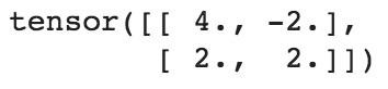
Notice that the gradients obtained previously match with the intuitive gradient values (which are two times that of the value of x).

By now, we have learned about initializing, manipulating, and calculating gradients on top of a tensor object – which together constitute the fundamental building blocks of a neural network. Except for calculating auto gradients, initializing and manipulating data can also be performed using NumPy arrays. This calls for us to understand the reason why you should use tensor objects over NumPy arrays when building a neural network – which we will go through in the next section.

Advantages of PyTorch's tensors over NumPy's ndarrays

In the previous chapter, we saw that when calculating the optimal weight values, we vary each weight by a small amount and understand its impact on reducing the overall loss value. Note that the loss calculation based on the weight update of one weight does not impact the loss calculation of the weight update of other weights in the same iteration. Thus, this process can be optimized if each weight update is being made by a different core in parallel instead of updating weights sequentially. A GPU comes in handy in this scenario as it consists of thousands of cores when compared to a CPU (which, in general, could have <=64 cores).

A Torch tensor object is optimized to work with a GPU compared to NumPy. To understand this further, let's perform a small experiment, where we perform the operation of matrix multiplication using NumPy arrays in one scenario and tensor objects in another and compare the time taken to perform matrix multiplication in both scenarios:

1. Generate two different torch objects:

import torch
x = torch.rand(1, 6400)
y = torch.rand(6400, 5000)

2. Define the device to which we will store the tensor objects we created in step 1:

device = 'cuda' if torch.cuda.is_available() else 'cpu'

3. Register the tensor objects that were created in step 1 with the device. Registering tensor objects means storing information in a device:

x, y = x.to(device), y.to(device)

4. Perform matrix multiplication of the Torch objects and also, time it so that we can compare the speed in a scenario where matrix multiplication is performed on NumPy arrays:

%timeit z=(x@y)
# It takes 0.515 milli seconds on an average to 
# perform matrix multiplication

5. Perform matrix multiplication of the same tensors on cpu:

x, y = x.cpu(), y.cpu()
%timeit z=(x@y)
# It takes 9 milli seconds on an average to 
# perform matrix multiplication

6. Perform the same matrix multiplication, this time on NumPy arrays:

import numpy as np
x = np.random.random((1, 6400))
y = np.random.random((6400, 5000))
%timeit z = np.matmul(x,y)
# It takes 19 milli seconds on an average to 
# perform matrix multiplication

You will notice that the matrix multiplication performed on Torch objects on a GPU is ~18X faster than Torch objects on a CPU, and ~40X faster than the matrix multiplication performed on NumPy arrays. In general, matmul with Torch tensors on a CPU is still faster than NumPy. Note that you would notice this kind of speed up only if you have a GPU device. If you are working on a CPU device, you would not notice the dramatic increase in speed. This is why if you do not own a GPU, we recommend using Google Colab notebooks, as the service provides free GPUs.

Now that we have learned how tensor objects are leveraged across the various individual components/operations of a neural network and how using the GPU can speed up computation, in the next section, we will learn about putting this all together to build a neural network using PyTorch.

Building a neural network using PyTorch

In the previous chapter, we learned about building a neural network from scratch, where the components of a neural network are as follows:

• The number of hidden layers
• The number of units in a hidden layer
• Activation functions performed at the various layers
• The loss function that we try to optimize for
• The learning rate associated with the neural network
• The batch size of data leveraged to build the neural network
• The number of epochs of forward and back-propagation

However, for all of these, we built them from scratch using NumPy arrays in Python. In this section, we will learn about implementing all of these using PyTorch on a toy dataset. Note that we will leverage our learning so far regarding initializing tensor objects, performing various operations on top of them, and calculating the gradient values to update weights when building a neural network using PyTorch.

The toy problem we'll solve to understand the implementation of neural networks using PyTorch is a plain addition of two numbers, where we initialize the dataset as follows:

1. Define the input (x) and output (y) values:

import torch
x = [[1,2],[3,4],[5,6],[7,8]]
y = [[3],[7],[11],[15]]

Note that in the preceding input and output variable initialization, the input and output are a list of lists where the sum of values in the input list is the values in the output list.

2. Convert the input lists into tensor objects:

X = torch.tensor(x).float()
Y = torch.tensor(y).float()

Note that in the preceding code, we have converted the tensor objects into floating-point objects. It is good practice to have tensor objects as floats or long ints, as they will be multiplied by decimal values (weights) anyway.

Furthermore, we register the input (X) and output (Y) data points to the device – cuda if you have a GPU and cpu if you don't have a GPU:

device = 'cuda' if torch.cuda.is_available() else 'cpu'
X = X.to(device)
Y = Y.to(device)

3. Define the neural network architecture:

• The torch.nn module contains functions that help in building neural network models:

import torch.nn as nn

• We will create a class (MyNeuralNet) that can compose our neural network architecture. It is mandatory to inherit from nn.Module when creating a model architecture as it is the base class for all neural network modules:

class MyNeuralNet(nn.Module):

• Within the class, we initialize all the components of a neural network using the __init__ method. We should call super().__init__() to ensure that the class inherits nn.Module:

def __init__(self):
    super().__init__()

With the preceding code, by specifying super().__init__(), we are now able to take advantage of all the pre-built functionalities that have been written for nn.Module. The components that are going to be initialized in the init method will be used across different methods in the MyNeuralNet class.

• Define the layers in the neural network:

    self.input_to_hidden_layer = nn.Linear(2,8)
    self.hidden_layer_activation = nn.ReLU()
    self.hidden_to_output_layer = nn.Linear(8,1)

In the preceding lines of code, we specified all the layers of neural network – a linear layer (self.input_to_hidden_layer), followed by ReLU activation (self.hidden_layer_activation), and finally, a linear layer (self.hidden_to_output_layer). Note that, for now, the choice of the number of layers and activation is arbitrary. We'll learn about the impact of the number of units in layers and layer activations in more detail in the next chapter.

• Furthermore, let's understand what the functions in the preceding code are doing by printing the output of the nn.Linear method:

# NOTE - This line of code is not a part of model building, 
# this is used only for illustration of Linear method
print(nn.Linear(2, 7))
Linear(in_features=2, out_features=7, bias=True)

In the preceding code, the linear method takes two values as input and outputs seven values, and also has a bias parameter associated with it. Furthermore, nn.ReLU() invokes the ReLU activation, which can then be used in other methods.

Some of the other commonly used activation functions are as follows:

• Sigmoid
• Softmax
• Tanh

Now that we have defined the components of a neural network, let's connect the components together while defining the forward propagation of the network:

    def forward(self, x):
        x = self.input_to_hidden_layer(x)
        x = self.hidden_layer_activation(x)
        x = self.hidden_to_output_layer(x)
        return x

By now, we have built the model architecture; let's inspect the randomly initialized weight values in the next step.

4. You can access the initial weights of each of the components by performing the following steps:

• Create an instance of the MyNeuralNet class object that we defined earlier and register it to device:

mynet = MyNeuralNet().to(device)

• The weights and bias of each layer can be accessed by specifying the following:

# NOTE - This line of code is not a part of model building, 
# this is used only for illustration of 
# how to obtain parameters of a given layer
mynet.input_to_hidden_layer.weight

The output of the preceding code is as follows:

• All the parameters of a neural network can be obtained by using the following code:

# NOTE - This line of code is not a part of model building, 
# this is used only for illustration of 
# how to obtain parameters of all layers in a model
mynet.parameters()

The preceding code returns a generator object.

• Finally, the parameters are obtained by looping through the generator, as follows:

# NOTE - This line of code is not a part of model building, 
# this is used only for illustration of how to 
# obtain parameters of all layers in a model 
# by looping through the generator object
for par in mynet.parameters():
    print(par)

The preceding code results in the following output:

• An alternative way of defining the model using the nn.Parameter function is as follows:

# for illustration only
class MyNeuralNet(nn.Module):
     def __init__(self):
        super().__init__()
        self.input_to_hidden_layer = nn.Parameter(
                                          torch.rand(2,8))
        self.hidden_layer_activation = nn.ReLU()
        self.hidden_to_output_layer = nn.Parameter(
                                          torch.rand(8,1))

     def forward(self, x):
        x = x @ self.input_to_hidden_layer
        x = self.hidden_layer_activation(x)
        x = x @ self.hidden_to_output_layer
        return x

5. Define the loss function that we optimize for. Given that we are predicting for a continuous output, we'll optimize for mean squared error:

loss_func = nn.MSELoss()

• The loss value of a neural network can be calculated by passing the input values through the neuralnet object and then calculating MSELoss for the given inputs:

_Y = mynet(X)
loss_value = loss_func(_Y,Y)
print(loss_value)
# tensor(91.5550, grad_fn=<MseLossBackward>)
# Note that loss value can differ in your instance 
# due to a different random weight initialization

In the preceding code, mynet(X) calculates the output values when the input is passed through the neural network. Furthermore, the loss_func function calculates the MSELoss value corresponding to the prediction of the neural network (_Y) and the actual values (Y).

Now that we have defined the loss function, we will define the optimizer that tries to reduce the loss value. The input to the optimizer will be the parameters (weights and biases) corresponding to the neural network and the learning rate when updating the weights.

For this instance, we will consider the stochastic gradient descent (more on different optimizers and the impact of the learning rate in the next chapter).

6. Import the SGD method from the torch.optim module and then pass the neural network object (mynet) and learning rate (lr) as parameters to the SGD method:

from torch.optim import SGD
opt = SGD(mynet.parameters(), lr = 0.001)

7. Perform all the steps to be done in an epoch together:

• Calculate the loss value corresponding to the given input and output.
• Calculate the gradient corresponding to each parameter.
• Update the weights based on the learning rate and gradient of each parameter.
• Once the weights are updated, ensure that the gradients that have been calculated in the previous step are flushed before calculating the gradients in the next epoch:

# NOTE - This line of code is not a part of model building, 
# this is used only for illustration of how we perform 
opt.zero_grad() # flush the previous epoch's gradients
loss_value = loss_func(mynet(X),Y) # compute loss
loss_value.backward() # perform back-propagation
opt.step() # update the weights according to the gradients computed

• Repeat the preceding steps as many times as the number of epochs using a for loop. In the following example, we are performing the weight update process for a total of 50 epochs. Furthermore, we are storing the loss value in each epoch in the list – loss_history:

loss_history = []
for _ in range(50):
    opt.zero_grad()
    loss_value = loss_func(mynet(X),Y)
    loss_value.backward()
    opt.step()
    loss_history.append(loss_value)

• Let's plot the variation in loss over increasing epochs (as we saw in the previous chapter, we update weights in such a way that the overall loss value decreases with increasing epochs):

import matplotlib.pyplot as plt
%matplotlib inline
plt.plot(loss_history)
plt.title('Loss variation over increasing epochs')
plt.xlabel('epochs')
plt.ylabel('loss value')

The preceding code results in the following plot:

Note that, as expected, the loss value decreases over increasing epochs.

So far, in this section, we have updated the weights of a neural network by calculating the loss based on all the data points provided in the input dataset. In the next section, we will learn about the advantage of using only a sample of input data points per weight update.

Dataset, DataLoader, and batch size

One hyperparameter in a neural network that we have not considered yet is the batch size. Batch size refers to the number of data points considered to calculate the loss value or update weights.

This hyperparameter especially comes in handy in scenarios where there are millions of data points, and using all of them for one instance of weight update is not optimal, as memory is not available to hold so much information. In addition, a sample can be representative enough of the data. Batch size helps in fetching multiple samples of data that are representative enough, but not necessarily 100% representative of the total data.

In this section, we will come up with a way to specify the batch size to be considered when calculating the gradient of weights, to update weights, which is in turn used to calculate the updated loss value:

1. Import the methods that help in loading data and dealing with datasets:

from torch.utils.data import Dataset, DataLoader
import torch
import torch.nn as nn

2. Import the data, convert the data into floating-point numbers, and register them to a device:

• Provide the data points to work on:

x = [[1,2],[3,4],[5,6],[7,8]]
y = [[3],[7],[11],[15]]

• Convert the data into floating-point numbers:

X = torch.tensor(x).float()
Y = torch.tensor(y).float()

• Register data to the device – given that we are working on a GPU, we specify that the device is 'cuda'. If you are working on a CPU, specify the device as 'cpu':

device = 'cuda' if torch.cuda.is_available() else 'cpu'
X = X.to(device)
Y = Y.to(device)

3. Instantiate a class of the dataset – MyDataset:

class MyDataset(Dataset):

Within the MyDataset class, we store the information to fetch one data point at a time so that a batch of data points can be bundled together (using DataLoader) and be sent through one forward and one back-propagation in order to update the weights:

• Define an __init__ method that takes input and output pairs and converts them into Torch float objects:

    def __init__(self,x,y):
        self.x = torch.tensor(x).float()
        self.y = torch.tensor(y).float()

• Specify the length (__len__) of the input dataset:

    def __len__(self):
        return len(self.x)

• Finally, the __getitem__ method is used to fetch a specific row:

    def __getitem__(self, ix):
        return self.x[ix], self.y[ix]

In the preceding code, ix refers to the index of the row that is to be fetched from the dataset.

4. Create an instance of the defined class:

ds = MyDataset(X, Y)

5. Pass the dataset instance defined previously through DataLoader to fetch the batch_size number of data points from the original input and output tensor objects:

dl = DataLoader(ds, batch_size=2, shuffle=True)

In addition, in the preceding code, we also specify that we fetch a random sample (by mentioning that shuffle=True) of two data points (by mentioning batch_size=2) from the original input dataset (ds).

• To fetch the batches from dl, we loop through it:

# NOTE - This line of code is not a part of model building, 
# this is used only for illustration of 
# how to print the input and output batches of data
for x,y in dl:
    print(x,y)

This results in the following output:

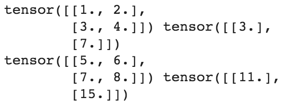
Note that the preceding code resulted in two sets of input-output pairs as there were a total of four data points in the original dataset, while the batch size that was specified was 2.

6. Now, we define the neural network class as we defined in the previous section:

class MyNeuralNet(nn.Module):
    def __init__(self):
        super().__init__()
        self.input_to_hidden_layer = nn.Linear(2,8)
        self.hidden_layer_activation = nn.ReLU()
        self.hidden_to_output_layer = nn.Linear(8,1)
    def forward(self, x):
        x = self.input_to_hidden_layer(x)
        x = self.hidden_layer_activation(x)
        x = self.hidden_to_output_layer(x)
        return x

7. Next, we define the model object (mynet), loss function (loss_func), and optimizer (opt) too, as defined in the previous section:

mynet = MyNeuralNet().to(device)
loss_func = nn.MSELoss()
from torch.optim import SGD
opt = SGD(mynet.parameters(), lr = 0.001)

8. Finally, loop through the batches of data points to minimize the loss value, just like we did in step 6 in the previous section:

import time
loss_history = []
start = time.time()
for _ in range(50):
    for data in dl:
        x, y = data
        opt.zero_grad()
        loss_value = loss_func(mynet(x),y)
        loss_value.backward()
        opt.step()
        loss_history.append(loss_value)
end = time.time()
print(end - start)

Note that while the preceding code seems very similar to the code that we went through in the previous section, we are performing 2X the number of weight updates per epoch when compared to the number of times the weights were updated in the previous section, as the batch size in this section is 2 whereas the batch size was 4 (the total number of data points) in the previous section.

Now that we have trained a model, in the next section, we will learn about predicting on a new set of data points.

Predicting on new data points

In the previous section, we learned how to fit a model on known data points. In this section, we will learn how to leverage the forward method defined in the trained mynet model from the previous section to predict on unseen data points. We will continue on from the code built in the previous section:

1. Create the data points that we want to test our model on:

val_x = [[10,11]]

Note that the new dataset (val_x) will also be a list of lists, as the input dataset was a list of lists.

2. Convert the new data points into a tensor float object and register to the device:

val_x = torch.tensor(val_x).float().to(device)

3. Pass the tensor object through the trained neural network – mynet – as if it were a Python function. This is the same as performing a forward propagation through the model that was built:

mynet(val_x)
# 20.99

The preceding code returns the predicted output values associated with the input data points.

By now, we have been able to train our neural network to map an input with output where we updated weight values by performing back-propagation to minimize the loss value (which is calculated using a pre-defined loss function).

In the next section, we will learn about building our own custom loss function instead of using a pre-defined loss function.

Implementing a custom loss function

In certain cases, we might have to implement a loss function that is customized to the problem we are solving – especially in complex use cases involving object detection/generative adversial networks (GANs). PyTorch provides the functionalities for us to build a custom loss function by writing a function of our own.

In this section, we will implement a custom loss function that does the same job as that of the MSELoss function that comes pre-built within nn.Module:

1. Import the data, build the dataset and DataLoader, and define a neural network, as done in the previous section:

x = [[1,2],[3,4],[5,6],[7,8]]
y = [[3],[7],[11],[15]]
import torch
X = torch.tensor(x).float()
Y = torch.tensor(y).float()
import torch.nn as nn
device = 'cuda' if torch.cuda.is_available() else 'cpu'
X = X.to(device)
Y = Y.to(device) 
import torch.nn as nn
from torch.utils.data import Dataset, DataLoader
class MyDataset(Dataset):
    def __init__(self,x,y):
        self.x = torch.tensor(x).float()
        self.y = torch.tensor(y).float()
    def __len__(self):
        return len(self.x)
    def __getitem__(self, ix):
        return self.x[ix], self.y[ix]
ds = MyDataset(X, Y)
dl = DataLoader(ds, batch_size=2, shuffle=True)
class MyNeuralNet(nn.Module):
    def __init__(self):
        super().__init__()
        self.input_to_hidden_layer = nn.Linear(2,8)
        self.hidden_layer_activation = nn.ReLU()
        self.hidden_to_output_layer = nn.Linear(8,1)
    def forward(self, x):
        x = self.input_to_hidden_layer(x)
        x = self.hidden_layer_activation(x)
        x = self.hidden_to_output_layer(x)
        return x
mynet = MyNeuralNet().to(device)

2. Define the custom loss function by taking two tensor objects as input, take their difference, and square them up and return the mean value of the squared difference between the two:

def my_mean_squared_error(_y, y):
    loss = (_y-y)**2
    loss = loss.mean()
    return loss

3. For the same input and output combination that we had in the previous section, nn.MSELoss is used in fetching the mean squared error loss, as follows:

loss_func = nn.MSELoss()
loss_value = loss_func(mynet(X),Y)
print(loss_value)
# 92.7534

my_mean_squared_error(mynet(X),Y)
# 92.7534

Notice that the results match. We have used the built-in MSELoss function and compared its result with the custom function that we built.

We can define a custom function of our choice, depending on the problem we are solving.

In the sections so far, we have learned about calculating the output at the last layer. The intermediate layer values have been a black box so far. In the next section, we will learn about fetching the intermediate layer values of a neural network.

Fetching the values of intermediate layers

In certain scenarios, it is helpful to fetch the intermediate layer values of the neural network (more on this when we discuss the style transfer and transfer learning use cases in later chapters).

PyTorch provides the functionality to fetch the intermediate values of the neural network in two ways:

• One way is by directly calling layers as if they are functions. This can be done as follows:

input_to_hidden = mynet.input_to_hidden_layer(X)
hidden_activation = mynet.hidden_layer_activation(
                                        input_to_hidden)
print(hidden_activation)

Note that we had to call the input_to_hidden_layer activation prior to calling hidden_layer_activation as the output of input_to_hidden_layer is the input to the hidden_layer_activation layer.

Let's look at the hidden layer values after activation for the model we have been working on in this chapter.

While all of the following code remains the same as what we saw in the previous section, we have ensured that the forward method returns not only the output but also the hidden layer values post-activation (hidden2):

class neuralnet(nn.Module):
    def __init__(self):
        super().__init__()
        self.input_to_hidden_layer = nn.Linear(2,8)
        self.hidden_layer_activation = nn.ReLU()
        self.hidden_to_output_layer = nn.Linear(8,1)
    def forward(self, x):
        hidden1 = self.input_to_hidden_layer(x)
        hidden2 = self.hidden_layer_activation(hidden1)
        output = self.hidden_to_output_layer(hidden2)
        return output, hidden2

mynet = neuralnet().to(device)
mynet(X)[1]

So far, we have learned about implementing a neural network using the class of neural networks where we manually built each layer. However, unless we are building a complicated network, the steps to build a neural network architecture are straightforward, where we specify the layers and the sequence with which layers are to be stacked. In the next section, we will learn about a simpler way of defining neural network architecture.

Using a sequential method to build a neural network

So far, we have built a neural network by defining a class where we define the layers and how the layers are connected with each other. In this section, we will learn about a simplified way of defining the neural network architecture using the Sequential class. We will perform the same steps as we have done in the previous sections, except that the class that was used to define the neural network architecture manually will be substituted with a Sequential class for creating a neural network architecture.

Let's code up the network for the same toy data that we have worked on in this chapter:

1. Define the toy dataset:

x = [[1,2],[3,4],[5,6],[7,8]]
y = [[3],[7],[11],[15]]

import torch
import torch.nn as nn
import numpy as np
from torch.utils.data import Dataset, DataLoader
device = 'cuda' if torch.cuda.is_available() else 'cpu'

class MyDataset(Dataset):
    def __init__(self, x, y):
        self.x = torch.tensor(x).float().to(device)
        self.y = torch.tensor(y).float().to(device)
    def __getitem__(self, ix):
        return self.x[ix], self.y[ix]
    def __len__(self): 
        return len(self.x)

4. Define the dataset (ds) and dataloader (dl) object:

ds = MyDataset(x, y)
dl = DataLoader(ds, batch_size=2, shuffle=True)

5. Define the model architecture using the Sequential method available in the nn package:

model = nn.Sequential(
            nn.Linear(2, 8),
            nn.ReLU(),
            nn.Linear(8, 1)
        ).to(device)

Note that, in the preceding code, we defined the same architecture of the network as we defined in previous sections, but defined differently. nn.Linear accepts two-dimensional input and gives an eight-dimensional output for each data point. Furthermore, nn.ReLU performs ReLU activation on top of the eight-dimensional output and finally, the eight-dimensional input gives a one-dimensional output (which in our case is the output of the addition of the two inputs) using the final nn.Linear layer.

6. Print a summary of the model we defined in step 5:

• Install and import the package that enables us to print the model summary:

!pip install torch_summary
from torchsummary import summary

• Print a summary of the model, which expects the name of the model and also the input size of the model:

summary(model, torch.zeros(1,2))

The preceding code gives the following output:

Note that the output shape of the first layer is (-1, 8), where -1 represents that there can be as many data points as the batch size, and 8 represents that for each data point, we have an eight-dimensional output resulting in an output of the shape batch size x 8. The interpretation for the next two layers is similar.

7. Next, we define the loss function (loss_func) and optimizer (opt) and train the model, just like we did in the previous section. Note that, in this case, we need not define a model object; a network is not defined within a class in this scenario:

loss_func = nn.MSELoss()
from torch.optim import SGD
opt = SGD(model.parameters(), lr = 0.001)
import time
loss_history = []
start = time.time()
for _ in range(50):
    for ix, iy in dl:
        opt.zero_grad()
        loss_value = loss_func(model(ix),iy)
        loss_value.backward()
        opt.step()
        loss_history.append(loss_value)
end = time.time()
print(end - start)

8. Now that we have trained the model, we can predict values on a validation dataset that we define now:

• Define the validation dataset:

val = [[8,9],[10,11],[1.5,2.5]]

• Predict the output of passing the validation list through the model (note that the expected value is the summation of the two inputs for each list within the list of lists). As defined in the dataset class, we first convert the list of lists into a float after converting them into a tensor object and registering them to the device:

model(torch.tensor(val).float().to(device))
# tensor([[16.9051], [20.8352], [ 4.0773]], 
# device='cuda:0', grad_fn=<AddmmBackward>)

Note that the output of the preceding code, as shown in the comment, is close to what is expected (which is the summation of the input values).

Now that we have learned about leveraging the sequential method to define and train a model, in the next section, we will learn about saving and loading a model to make an inference.

Saving and loading a PyTorch model

One of the important aspects of working on neural network models is to save and load back a model after training. Think of a scenario where you have to make inferences from an already-trained model. You would load the trained model instead of training it again.

Before going through the relevant commands to do that, taking the preceding example as our case, let's understand what all the important components that completely define a neural network are. We need the following:

• A unique name (key) for each tensor (parameter)
• The logic to connect every tensor in the network with one or the other
• The values (weight/bias values) of each tensor

While the first point is taken care of during the __init__ phase of a definition, the second point is taken care of during the forward method definition. By default, the values in a tensor are randomly initialized during the __init__ phase. But what we want is to load a specific set of weights (or values) that were learned when training a model and associate each value with a specific name. This is what you obtain by calling a special method, described in the following sections.

state dict

The model.state_dict() command is at the root of understanding how saving and loading PyTorch models works. The dictionary in model.state_dict() corresponds to the parameter names (keys) and the values (weight and bias values) corresponding to the model. state refers to the current snapshot of the model (where the snapshot is the set of values at each tensor).

It returns a dictionary (OrderedDict) of keys and values:

The keys are the names of the model's layers and the values correspond to the weights of these layers.

Saving

Running torch.save(model.state_dict(), 'mymodel.pth') will save this model in a Python serialized format on the disk with the name mymodel.pth. A good practice is to transfer the model to the CPU before calling torch.save as this will save tensors as CPU tensors and not as CUDA tensors. This will help in loading the model onto any machine, whether it contains CUDA capabilities or not.

We save the model using the following code:

torch.save(model.to('cpu').state_dict(), 'mymodel.pth')

Now that we understand saving a model, in the next section, we will learn about loading the model.

Loading

Loading a model would require us to initialize the model with random weights first and then load the weights from state_dict:

1. Create an empty model with the same command that was used in the first place when training:

model = nn.Sequential(
            nn.Linear(2, 8),
            nn.ReLU(),
            nn.Linear(8, 1)
        ).to(device)

2. Load the model from disk and unserialize it to create an orderedDict value:

state_dict = torch.load('mymodel.pth')

3. Load state_dict onto model, register to device, and make a prediction:

model.load_state_dict(state_dict)
# <All keys matched successfully>
model.to(device)
model(torch.tensor(val).float().to(device))

If all the weight names are present in the model, then you would get a message saying all the keys were matched. This implies we are able to load our model from disk, for all purposes, on any machine in the world.

Next, we can register the model to the device and perform inference on the new data points, as we learned in the previous section.

Summary

In this chapter, we learned about the building blocks of PyTorch – tensor objects and performing various operations on top of them. We proceeded further by building a neural network on a toy dataset where we started by building a class that initializes the feed-forward architecture, fetching data points from the dataset by specifying the batch size, and defining the loss function and the optimizer, looping through multiple epochs. Finally, we also learned about defining custom loss functions to optimize a metric of choice and leveraging the sequential method to simplify the process of defining the network architecture.

All the preceding steps form the foundation of building a neural network, which will be leveraged multiple times in the various use cases that we will build in subsequent chapters.

With this knowledge of the various components of building a neural network using PyTorch, we will proceed to the next chapter, where we will learn about the various practical aspects of dealing with the hyperparameters of a neural network on image datasets.

Questions

1. Why should we convert integer inputs into float values during training?
2. What are the various methods to reshape a tensor object?
3. Why is computation faster with tensor objects over NumPy arrays?
4. What constitutes the init magic function in a neural network class?
5. Why do we perform zero gradients before performing back-propagation?
6. What magic functions constitute the dataset class?
7. How do we make predictions on new data points?
8. How do we fetch the intermediate layer values of a neural network?
9. How does the sequential method help in simplifying defining the architecture of a neural network?