
2
Minimum Common String Partition Problem
This chapter deals with a combinatorial optimization (CO) problem from computational biology known as the unbalanced minimum common string partition (UMCSP) problem. The UMCSP problem includes the minimum common string partition (MCSP) problem as a special case. First, an ILP model for the UMCSP problem is described. Second, a greedy heuristic initially introduced for the MCSP problem is adapted for application to the UMCSP problem. Third, the application of a general hybrid metaheuristic labeled construct, merge, solve and adapt (CMSA) to the UMCSP problem is described. The CMSA algorithm is based on the following principles. At each iteration, the incumbent sub-instance is modified by adding solution components found in probabilistically constructed solutions to the problem tackled. Moreover, the incumbent sub-instance is solved to optimality (if possible) by means of an ILP solver such as CPLEX. Finally, seemingly useless solution components are removed from the incumbent sub-instance based on an ageing mechanism. The results obtained indicate that the CMSA algorithm outperforms the greedy approach. Moreover, they show that the CMSA algorithm is competitive with CPLEX for small and medium problems, whereas it outperforms CPLEX for larger problems. Note that this chapter is based on [BLU 13].
2.1. The MCSP problem
Given that the special case – that is, the MCSP problem – is easier to describe than the UMCSP, we will first describe the MCSP problem. The MCSP problem was introduced in [CHE 05] due to its association with genome rearrangement. It has applications in biological questions such as: may a given DNA string be obtained by rearranging another DNA string? There are two input strings s1 and s2 of length n over a finite alphabet Σ. The two strings need to be related, which means that each letter appears the same number of times in each of them. This definition implies that s1 and s2 are the same length n. A valid solution to the MCSP problem is obtained by partitioning s1 into a set P1 of non-overlapping substrings, and s2 into a set P2 of non-overlapping substrings, such that P1 = P2. Moreover, the goal is to find a valid solution such that |P1| = |P2| is minimum.
Consider the following example with the DNA sequences s1 = AGACTG and s2 = ACTAGG. As A and G appear twice in both input strings, and C and T appear once, the two strings are related. A trivial valid solution can be obtained by partitioning both strings into substrings of length 1, i.e. P1 = P2 = {A, A, C, T, G, G}. The objective function value of this solution is 6. However, the optimal solution, with objective function value 3, is P1 = P2 = {ACT, AG, G}.
2.1.1. Technical description of the UMCSP problem
The more general UMCSP problem [BUL 13] can technically be described as follows with an input string s1 of length n1 and an input string s2 of length n2, both over the same finite alphabet Σ. A valid solution to the UMCSP problem is obtained by partitioning s1 into a set P1 of non-overlapping substrings, and s2 into a set P2 of non-overlapping substrings, such that a subset S1 ⊆ P1 and a subset S2 ⊆ P2 exist with S1 = S2 and no letter a ∈ Σ is simultaneously present in a string x ∈ P1 S1 and a string y ∈ P2 S2. Henceforth, given P1 and P2, let us denote the largest subset S1 = S2 such that the above-mentioned condition holds by S∗. The objective function value of solution (P1, P2) is then |S∗|. The goal consists of finding solution (P1, P2) where |S∗| is minimum.
Consider the following example with the DNA sequences s1 = AAGACTG and s2 = TACTAG. Again, a trivial valid solution can be obtained by partitioning both strings into substrings of length 1, i.e. P1 = {A, A, A, C, T, G, G} and P2 = {A, A, C, T, T, G}. In this case, S∗ = {A, A, C, T, G}, and the objective function value is |S∗| = 5. However, the optimal solution, with objective function value 2, is P1 = {ACT, AG, A, G}, P2 = {ACT, AG, T} and S∗ = {ACT, AG}.
Note that the only difference between the UMCSP and the MCSP is that the UMCSP does not require the input strings to be related.
2.1.2. Literature review
The MCSP problem that was first studied in the literature, has been shown to be non-deteministic polynomial time (NP)-hard even in very restrictive cases [GOL 05]. The MCSP has been considered quite extensively by researchers dealing with the approximability of the problem. In [COR 07], for example, the authors proposed an O(log n log∗ n)-approximation for the edit distance with moves problem, which is a more general case of the MCSP problem. Shapira and Storer [SHA 02] extended this result. Other approximation approaches to the MCSP problem have been proposed in [KOL 07]. In this context, the authors of [CHR 04] studied a simple greedy approach to the MCSP problem, showing that the approximation ratio concerning the 2-MCSP problem is 3 and for the 4-MCSP problem the approximation ratio is Ω(log n). Note, in this context, that the notation k-MCSP refers to a restricted version of the MCSP problem in which each letter occurs at most k times in the input strings. In case of the general MCSP problem, the approximation ratio is between Ω(n0.43) and O(n0.67), assuming that the input strings use an alphabet of size O(log n). Later, in [KAP 06] the lower bound was raised to Ω(n0.46). The authors of [KOL 05] proposed a modified version of the simple greedy algorithm with an approximation ratio of O(k2) for the k-MCSP. Recently, the authors of [GOL 11] proposed a greedy algorithm for the MCSP problem that runs in O(n) time. Finally, in [HE 07] a greedy algorithm aiming to obtain better average results was introduced.
The first ILP model for the MCSP problem, together with an ILP-based heuristic, was proposed in [BLU 15b]. Later, more efficient ILP models were proposed in [BLU 16d, FER 15]. Regarding metaheuristics, the MCSP problem has been tackled by the following approaches:
- 1) a MAX–MIN Ant System (MMAS) by Ferdous and Sohel Rahman [FER 13a, FER 14];
- 2) a probabilistic tree search algorithm by Blum et al. [BLU 14a].
- 3) a CMSA algorithm by Blum et al. [BLU 16b].
As mentioned above, the UMCSP problem [BUL 13] is a generalization of the MCSP problem [CHE 05]. In contrast to the MCSP, the UMCSP has not yet been tackled by means of heuristics or metaheuristics. The only existing algorithm is a fixed-parameter approximation algorithm described in [BUL 13].
2.1.3. Organization of this chapter
The remaining parts of the chapter is organized as follows. The first ILP model in the literature for the UMCSP problem is described in section 2.2. In section 2.4, the application of CMSA to the UMCSP problem is outlined. Finally, section 2.5 provides an extensive experimental evaluation and section 2.6 presents a discussion on promising future lines of research concerning UMCSP.
2.2. An ILP model for the UMCSP problem
As a first step in the development of an ILP model, the UMCSP problem is re-phrased by making use of the common block concept. Given input strings s1 and s2, a common block bi is denoted as a triplet ![]() , where ti is a string which can be found starting at position
, where ti is a string which can be found starting at position ![]() in string s1 and starting at position
in string s1 and starting at position ![]() in string s2. Let B = {b1, … , bm} be the complete set of common blocks. Moreover, let us assume that the blocks appear in B in no particular order. In addition, given a string t over alphabet Σ, let n(t, a) denote the number of occurrences of letter a ∈ Σ in t. That is n(s1, a), and respectively n(s2, a), denote the number of occurrences of letter a ∈ Σ in input string s1, and s2 respectively. Then, a subset S of B corresponds to a valid solution to the UMCSP problem if and only if the following conditions hold:
in string s2. Let B = {b1, … , bm} be the complete set of common blocks. Moreover, let us assume that the blocks appear in B in no particular order. In addition, given a string t over alphabet Σ, let n(t, a) denote the number of occurrences of letter a ∈ Σ in t. That is n(s1, a), and respectively n(s2, a), denote the number of occurrences of letter a ∈ Σ in input string s1, and s2 respectively. Then, a subset S of B corresponds to a valid solution to the UMCSP problem if and only if the following conditions hold:
- 1)
 bi∈S n(ti, a) = min{n(s1, a), n(s2, a)} for all a ∈ Σ. That is, the sum of the occurrences of a letter a ∈ Σ in the common blocks present in S must be less than or equal to the minimum number of occurrences of letter a in s1 and s2.
 - 2) For any two common blocks
 the corresponding strings do not overlap in s1 nor in s2.
A possible ILP model for the UMCSP problem for each common block bi ∈ B uses a binary variable xi, indicating whether or not the corresponding common block forms part of the solution. In other words, if xi = 1, the corresponding common block bi is selected for the solution, and if xi = 0, common block bi is not selected.
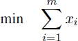
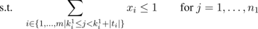
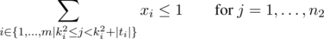
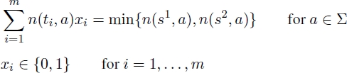
Objective function [2.1] minimizes the number of common blocks selected. Equations [2.2] ensure that the strings corresponding to the common blocks selected do not overlap with respect to s1 and equations [2.3] ensure the same with respect to s2. Finally, equations [2.4] ensure that the number of occurrences of each letter in the selected strings is equal to the minimum number of occurrences of this letter in s1 and s2.
2.3. Greedy approach
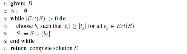
The following greedy heuristic, henceforth called GREEDY, is an extension of the greedy heuristic from [HE 07] which was introduced for the MCSP problem. It starts with the empty partial solution and chooses at each construction step exactly one common block and adds it to the valid partial solution under construction. Therefore, S ⊂ B is called a valid partial solution if the substrings corresponding to the common blocks in S do not overlap for s1 or s2. Furthermore, let set Ext(S) ⊂ B S denote the set of common blocks that may be used to extend S such that the result is again a valid (partial) solution. Note that when Ext(S) = ∅, S corresponds to a complete solution. At each step GREEDY chooses the common block with the longest substring from Ext(S). The pseudo-code of GREEDY is provided in Algorithm 2.1.
Algorithm 2.1. GREEDY
2.4. Construct, merge, solve and adapt
The drawback of exact solvers in the context of CO problems – especially for problems from computational biology – is often that they are not applicable to problems of realistic size. When small problems are considered, however, exact solvers are often extremely efficient. This is because a considerable amount of time, effort and expertise has gone into the development of exact solvers. Examples include general-purpose ILP solvers such as CPLEX and Gurobi. Having this in mind, recent research efforts have focused on ways of making use of exact solvers within heuristic frameworks even in the context of large problems. A recently-proposed algorithm labeled CMSA [BLU 16b, BLU 15a] falls into this line of research. A general description of this algorithm is provided in section 1.2.7.2. In short, the algorithm works as follows. At each iteration, solutions to the problem tackled are generated in a probabilistic way. The components found in these solutions are then added to an incumbent sub-instance of the original problem. Subsequently, an exact solver – CPLEX, in the case of this chapter – is used to optimally solve the incumbent sub-instance. Moreover, the algorithm makes use of a mechanism for deleting seemingly useless components from the incumbent sub-instance. This is done in order to prevent these solution components slowing down the exact solver when applied to the sub-instance.
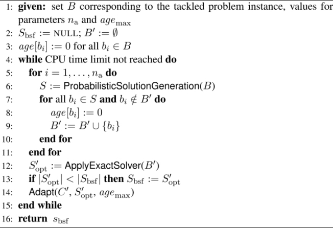
More specifically, the CMSA algorithm applied to the UMCSP problem, whose pseudo-code is given in Algorithm 2.2, works as follows. It maintains an incumbent sub-instance B′, which is a subset of the complete set B of common blocks. Moreover, each common block bi ∈ B has a non-negative age value denoted by age[bi]. At the start of the algorithm, the best-so-far solution Sbsf is set to NULL, indicating that no such solution yet exists, and the sub-instance B′ is set to the empty set. Then, at each iteration, a number of na solutions is probabilistically generated, see function ProbabilisticSolutionGeneration(B) in line 6 of Algorithm 2.2. The common blocks that form part of these solutions are added to B′ and their age is re-set to 0. Afterwards, the ILP solver CPLEX is applied to optimally solve sub-instance B′. Note that if this is not possible within the given CPU time limit, CPLEX simply returns the best solution found so far; see function ApplyExactSolver(B′ ) in line 12 of Algorithm 2.2. If S′opt is better than the current best-so-far solution Sbsf, solution S′opt replaces the best-so-far solution (line 13). Next, sub-instance B′ is updated. This is done based on solution S′opt and on the age values of the common blocks; see function Adapt(B′, S′opt, agemax) in line 14. The functions of this algorithm are comprehensively described in the following:
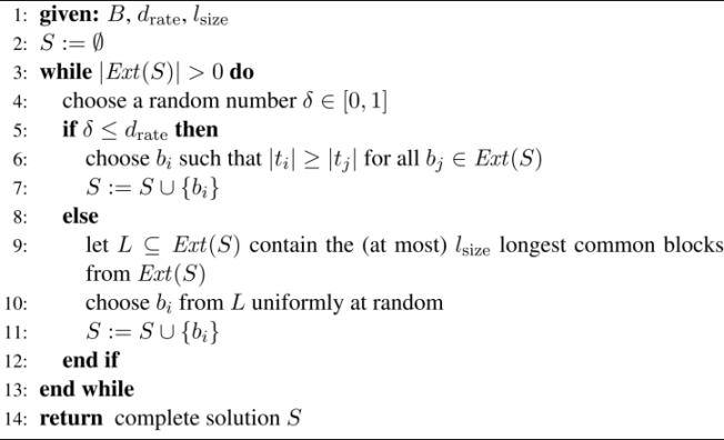
- – ProbabilisticSolutionGeneration(B) function: to generate a solution in a probabilistic way, this function (see line 6 of Algorithm 2.2) makes use of the GREEDY algorithm described in section 2.3. However, instead of choosing, at each construction step, the common block with maximum sub-string length from Ext(S), the choice of a common block bi ∈ Ext(S) is made as follows. First, a value δ ∈ [0, 1) is chosen uniformly at random. In case δ ≤ drate, bi is chosen such that |ti| ≥ |tj| for all bj ∈ Ext(S), i.e. one of the common blocks whose substring is of maximum size is chosen. Otherwise, a candidate list L containing the (at most) lsize longest common blocks from Ext(S) is built and bi is chosen from L uniformly at random. In other words, the greediness of this procedure depends on the values of two input parameters: (1) the determinism rate (drate); and (2) the candidate list size (lsize).
Algorithm 2.2. CMSA for the UMCSP problem
- – ApplyExactSolver(B′ ) function: CPLEX is used in order to find the best solution contained in a sub-instance B′. The ILP model outlined in section 2.2 is used for this purpose after replacing all occurrences of B in this ILP model with B′ and by replacing m with |B′ |.
- – Adapt(B′, S′opt, agemax) function: this function initially increases the age of all common blocks in B′ S′opt. Moreover, the age of all common blocks in S′opt ⊆ B′ is re-set to zero. Then, those common blocks from B′ whose age has reached the maximum component age (agemax) are deleted from B′. This removes common blocks that never form part of the optimal solution to B′ after some time in order to prevent them slowing down the ILP solver.
2.5. Experimental evaluation
We now present an experimental comparison between the two techniques presented so far in this chapter – namely GREEDY and CMSA. IBM ILOG CPLEX v12.2 is applied to each problem considered. The application of CPLEX is henceforth referred to as CPLEX. All code was implemented in ANSI C++ using GCC 4.7.3 to compile the software. In the context of CMSA and CPLEX, CPLEX was used in single-threaded mode. The experimental evaluation was performed on a cluster of PCs with Intel(R) Xeon(R) CPU 5670 CPUs of 12 nuclei of 2933 MHz and at least 40 GB of RAM. Note that the fixed- parameter approximation algorithm described in [BUL 13] was not included in the comparison because, according to the authors of this work, the algorithm is only applicable to very small problem.
In the following, first, the set of benchmarks that were generated to test the solution methods considered are described. Then, the tuning experiments that were performed in order to determine a proper setting for the parameters of CMSA are outlined. Finally, an exhaustive experimental evaluation is presented.
2.5.1. Benchmarks
A set of 600 benchmarks was generated for the comparison of the three solutions considered. The benchmark set consists of 10 randomly generated instances for each combination of base-length n ∈ {200, 400, … , } 1800, 2000}, alphabet size |Σ| ∈ {4, 12}, and length-difference ld ∈ {0, 10, 20}. Each letter of Σ has the same probability of appearing at any of positions in input strings s1 and s2. Given a value for the base-length n and the length-difference ld, the length of s1 is determined as ![]() and the length of s2 as
and the length of s2 as ![]() . In other words, ld refers to the difference in length between s1 and s2 (in percent) given a certain base-length, n.
. In other words, ld refers to the difference in length between s1 and s2 (in percent) given a certain base-length, n.
2.5.2. Tuning CMSA
There are several parameters involved in CMSA for which well-working values must be found: (na) the number of solution constructions per iteration, (agemax) the maximum allowed age of common blocks, (drate) the determinism rate, (lsize) the candidate list size, and (tmax) the maximum time in seconds allowed for CPLEX per application to a sub-instance. The last parameter is necessary, because even when applied to reduced problems, CPLEX might still need too much computation time to optimally solve such sub-instances. CPLEX always returns the best feasible solution found within the given computation time.
Table 2.1. Results of tuning CMSA for the UMCSP problem using irace
|
n |
na |
agemax |
drate |
lsize |
tmax |
|
200 |
50 |
10 |
0.0 |
10 |
480 |
|
400 |
50 |
10 |
0.0 |
10 |
120 |
|
600 |
50 |
10 |
0.0 |
10 |
240 |
|
800 |
50 |
5 |
0.5 |
10 |
120 |
|
1000 |
50 |
10 |
0.7 |
10 |
60 |
|
1200 |
50 |
5 |
0.5 |
10 |
120 |
|
1400 |
50 |
10 |
0.9 |
10 |
480 |
|
1600 |
50 |
5 |
0.9 |
10 |
480 |
|
1800 |
50 |
5 |
0.9 |
10 |
480 |
|
2000 |
50 |
10 |
0.9 |
10 |
480 |
The automatic configuration tool irace [LÓP 11] was used to tune the five parameters. In fact, irace was applied to tune separately CMSA for each base-length, which – after initial experiments – seemed to be the parameter with the most influence on algorithm performance. For each of the 10 base-length values considered, 12 tunings were randomly generated: two for each of the six combinations of Σ and ld. The tuning process for each alphabet size was given a budget of CMSA 1,000 runs, where each run was given a computation time limit of 3, 600 CPU seconds. Finally, the following parameter value ranges were chosen for the five parameters of CMSA:
- – na ∈ {10, 30, 50};
- – agemax ∈ {1, 5, 10, inf}, where inf means that no common block is ever removed from sub-instance B′;
- – where a value of 0.0 means that the selection of the next common block to be added to the partial solution under construction is always done randomly from the candidate list, while a value of 0.9 means that solution constructions are nearly deterministic;
- – lsize ∈ {3, 5, 10};
- – tmax ∈ {60, 120, 240, 480} (in seconds).
The tuning runs with irace produced the configurations of CMSA shown in Table 2.1. The most important tendencies that can be observed are the following ones. First, with growing base-length, the greediness of the solution constructed grows, as indicated by the increasing value of drate. Second, the number of solutions constructed per iteration is always high. Third, the time limit for CPLEX does not play any role for smaller instances. However, for larger instances the time limit of 480 seconds is consistently chosen.
2.5.3. Results
The numerical results concerning all instances with |Σ| = 4 are summarized in Table 2.2, and concerning all instances with |Σ| = 12 in Table 2.3. Each table row presents the results averaged over 10 problems of the same type. For each of the three methods in the comparison (at least) the first column (with the heading mean) provides the average values of the best solutions obtained over 10 problems, while the second column (time) provides the average computation time (in seconds) necessary to find the corresponding solutions. In the case of CPLEX, this column provides two values in the form X/Y, where X corresponds to the (average) time at which CPLEX was able to find the first valid solution, and Y to the (average) time at which CPLEX found the best solution within 3,600 CPU seconds. An additional column with the heading gap in the case of CPLEX provides the average optimality gaps (in percent), i.e. the average gaps between the upper bounds and the values of the best solutions when stopping a run. A third additional column in the case of CMSA (size (%)) provides the average size of the sub-instances considered in CMSA as a percentage of the original problem size, i.e. the sizes of the complete sets B of common blocks. Finally, note that the best result for each table row is marked with a gray background. The numerical results are presented graphically in Figures 2.1 and 2.2 in terms of the improvement of CMSA over CPLEX and GREEDY (in percent).
The results allow us to make the following observations:
- – applying CPLEX to the original problems, the alphabet size has a strong influence on the problem difficulty. Where |Σ| = 4, CPLEX is only able to provide feasible solutions within 3,600 CPU seconds for input string lengths of up to 800. When |Σ| = 12, CPLEX provides feasible solutions for input string lengths of up to 1,600 (for ld ∈ {0, 10}). When ld = 20, CPLEX is able to provide feasible solutions for all problem instances;
- – in contrast to CPLEX, CMSA provides feasible solutions for all problems. Moreover, CMSA outperforms GREEDY in all cases. In those cases in which CPLEX is able to provide feasible (or even optimal) solutions, CMSA is either competitive or not much worse than CPLEX. CMSA is never more than 3% worse than CPLEX.
Table 2.2. Results for instances where |Σ| = 4
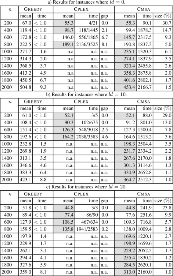
Table 2.3. Results for instances where |Σ| = 12
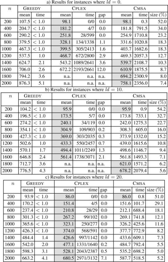
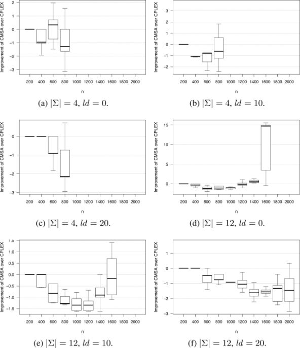
Figure 2.1. Improvement of CMSA over CPLEX (in percent). Note that when boxes are missing, CPLEX was not able to provide feasible solutions within the computation time allowed
In summary, CMSA is competitive when CPLEX is applied to the original ILP model when the size is rather small. The larger the size of the inputs, and the smaller the alphabet size, the greater the general advantage of CMSA over the other algorithms.
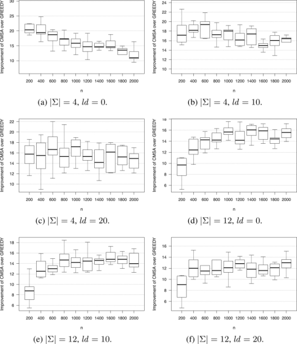
Figure 2.2. Improvement of CMSA over GREEDY (in percent)
Finally, the size of the sub-instances that are generated (and maintained) within CMSA in comparison to the size of the original problems are presented. These sub-instance sizes are provided in a graphical way in Figure 2.3. Note that these graphics show the sub-instance sizes averaged over all instances of the same alphabet size and the same ld value. In all cases, the x-axis ranges from instances with a small base-length (n) at the left, to instances with a large base-length at the right. Interestingly, when the base-length is rather small, the sub-instances tackled in CMSA are rather large (up to ≈ 55% of the size of the original problems). With growing base-length, the size of the sub-instances tackled decreases. The reason for this trend is as follows. As CPLEX is very efficient for problems created with rather small base-lengths, the parameter values of CMSA are chosen during the irace tuning process so that the sub-instance become quite large. With growing base-length, however, the parameter values chosen during tuning lead to smaller sub-instances, simply because CPLEX is not so efficient when applied to sub-instances that are not much smaller than the original problems.
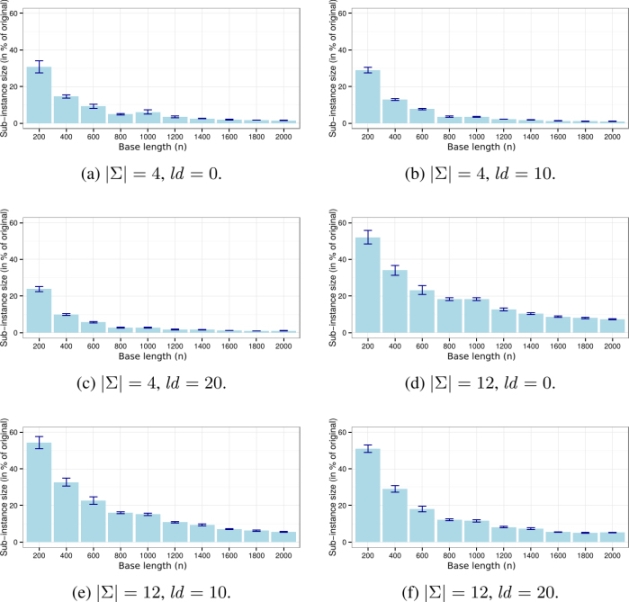
Figure 2.3. Graphical presentation of the sizes of the sub-instances as a percentage of the size of the original problems
2.6. Future work
For the UMCSP problem, pure metaheuristic approaches such as the MMAS algorithm from [FER 13a, FER 14] have been greatly outperformed by the application of CPLEX to the existing benchmarks. Understanding the reason for this will be an important step towards the development of pure metaheuristics – note that CMSA is a hybrid metaheuristic because it makes use of an ILP solver – for MCSP and UMCSP problems. This will be necessary as CPLEX and CMSA will reach their limits with growing problem size.