
5
Consensus String Problems
This chapter provides an overview of some string selection and comparison problems, with special emphasis on consensus string problems. The intrinsic properties of the problems are studied and the most popular solution techniques given, including some recently-proposed heuristic and metaheuristic approaches. Finally, a simple and efficient ILP-based heuristic that can be used for any of the problems considered is presented. Future directions are discussed in the last section.
5.1. Introduction
Among string selection and comparison problems there is a class of problems known as consensus string problems, where a finite set of strings is given and one is interested in finding their consensus, i.e. a new string that agrees as much as possible with all the given strings. In other words, the objective is to determine a consensus string that once one or more criteria have been defined represents all the given strings. The idea of consensus can be related to several different objectives and prospectives. Some of them are considered in this chapter and are listed in the following:
- 1) the consensus is a new string whose total distance from all given strings is minimal (closest string problem);
- 2) the consensus is a new string close to most of the given strings (close to most string problem);
- 3) the consensus is a new string whose total distance from all given strings is maximal (farthest string problem);
- 4) the consensus is a new string far from most of the given strings (far from most string problem).
As a result of the linear coding of DNA and proteins, many molecular biology problems have been formulated as computational optimization (CO) problems involving strings and consisting of computing distance/proximity. Some biological applications require a region of similarity be discovered, while other applications use the reverse complement of the region, such as the designing of probes or primers. In the following, some relevant biological applications are listed.
5.1.1. Creating diagnostic probes for bacterial infections
Probes are strands of either DNA or RNA that have been modified (i.e. made either radioactive or fluorescent) so that their presence can be easily detected. One possible application of string problems arises in creating diagnostic probes for bacterial infections [LAN 04, MAC 90]. In this scenario, given a set of DNA strings from a group of closely-related pathogenic bacteria, the task is to find a substring that occurs in each of the bacterial strings (that is as close as possible) without occurring in the host’s DNA. Probes are then designed to hybridize to these target strings, so that the detection of their presence indicates that at least one bacterial species is likely to be present in the host.
5.1.2. Primer design
Primers are short strings of nucleotides designed so that they hybridize to a given DNA string or to all of a given set of DNA strings with the aim of providing a starting point for DNA strand synthesis by polymerase chain reaction (PCR). The hybridization of primers depends on several conditions, including some thermodynamic rules, but it is largely influenced by the number of mismatching positions among the given strings, and this number should be as small as possible [GRA 03a, GRA 02, LI 99].
5.1.3. Discovering potential drug targets
Another biological application of string selection and comparison problems is related to discovering potential drug targets. Given a set of strings of orthologous genes from a group of closely-related pathogens, and a host (such as a human, crop, or livestock), the goal is to find a string fragment that is more conserved in all or most of the pathogens strings but not as conserved in the host. Information encoded by this fragment can then be used for novel antibiotic development or to create a drug that harms several pathogens with minimum effect on the host. All these applications involve finding a pattern that, with some error, occurs in one set of strings (closest string problem) and/or does not occur in another set (farthest string problem). The far from most string problem can help to identify a string fragment that distinguishes the pathogens from the host, so the potential exists to create a drug that harms several but not all pathogens [GRA 03a, GRA 02, LI 99].
5.1.4. Motif search
A motif is a string that is approximately preserved as a substring in some/several of the DNA strings of a given set. Approximately preserved means that the motif occurs with changes in at most t positions for a fixed non-negative integer t. The importance of a motif is that it is a candidate for substrings of non-coding parts of the DNA string that have functions related to, gene expression for instance [GRA 03a, GRA 02].
The general strings consensus problem was proved computationally intractable by Frances and Litman [FRA 97] and by Sim and Park [SIM 99, SIM 03]. For most consensus problems, Hamming distance is used instead of alternative measures, such as the editing distance. Given two strings s1 and s2 on an alphabet Σ: where ![]() denotes their Hamming distance and is given by
denotes their Hamming distance and is given by
where s1j and s2j denote the character at position j in string s1 and in string s2, respectively, and Φ : Σ × Σ → {0, 1} is a predicate function such that:
For all consensus problems, each string s of length m over Σ is a valid solution. The biological reasons justifying the choice of the Hamming distance are very well described and motivated by Lanctot et al. in [LAN 99, LAN 03, LAN 04] and can be summarized with the claim that the “edit distance is more suitable to measure the amount of change that has happened, whereas the Hamming distance is more suitable to measure the effect of that change”.
5.2. Organization of this chapter
The remainder of this chapter is organized as follows. Sections 5.3 and 5.4 are devoted to the closest string and the close to most string and the farthest string and the far from most string problem, respectively. All these problems are mathematically formulated and their properties analyzed. The most popular solutions are surveyed, along with the computational results obtained and analyzed in the literature. Section 5.5 describes a simple ILP-based heuristic that can be used for any of the problems considered. Concluding remarks and future directions are discussed in the last section.
5.3. The closest string problem and the close to most string problem
Given a finite set Ω of strings of length m over a finite alphabet Σ, the closest string problem (CSP) is to find a center string s* ∈ Σm such that the Hamming distance between s* and all strings in Ω is minimal; in other words, s* is a string to which a minimum value d corresponds such that:
The CSP can be seen as a special case of the close to most string problem (CTMSP), which consists of determining a string close to most of the strings in the input set Ω. This can be formalized by saying that, given a threshold t, a string s* must be found maximizing the variable l such that:
5.3.1. ILP models for the CSP and the CTMSP
Let Σk ⊆ Σ be the set of characters appearing at position k in any of the strings from Ω. The closest string problem can be formulated as an integer linear program (ILP) that uses k = 1, 2, … , m for each position and c ∈ Σk for each character, the following binary variables:
Then, the CSP can be formulated as follows:
Objective function [5.2] minimizes d, i.e. the right-hand side of inequalities [5.4] which mean that if a character in a string si is not in the solution defined by the x-variables, then that character will contribute to increasing the Hamming distance from solution x to si. In this context, remember that ![]() denotes the character at position k in si ∈ Ω. d is forced to assume a non-negative integer value by [5.5]. Equalities [5.3] guarantee that only one character is selected for each position k ∈ {1, 2, … , m}. Finally, [5.6] define the decision variables.
denotes the character at position k in si ∈ Ω. d is forced to assume a non-negative integer value by [5.5]. Equalities [5.3] guarantee that only one character is selected for each position k ∈ {1, 2, … , m}. Finally, [5.6] define the decision variables.
Besides the binary x-variables, to mathematically formulate the CTMSP a further binary vector y ∈ {0, 1}|Ω| is introduced and the resulting ILP model can be stated as:

Equalities [5.8] guarantee that only one character is selected for each position k ∈ {1, 2, … , m} for the CSP. Inequalities [5.4] ensure that yi can only be set to 1 if and only if the number of differences between si ∈ Ω and the possible solution (as defined by setting of the xck variables) is less than or equal than t. The objective function [5.7] maximizes the number of y-variables set to 1. Finally, [5.10] and [5.11] define the decision variables.
5.3.2. Literature review
The CSP was first studied in the area of coding theory [ROM 92] and has been independently proven to be computationally intractable in [FRA 97] and in [LAN 99, LAN 03].
Since then, few exact and approximation algorithms and several heuristic procedures have been proposed. Despite its similarity with the CSP, the CTMSP instead has not been widely studied. In [BOU 13] it was proven that this problem has no polynomial-time approximation scheme (PTAS)1 unless NP has randomized polynomial-time algorithms.
5.3.3. Exact approaches for the CSP
In 2004, Meneses et al. [PAR 04] used a linear relaxation of the ILP model of the problem to design a B&B algorithm. At each iteration, to generate the next node in the branching tree the best bound first strategy is adopted to select the next node and obtain an optimal fractional solution ![]()
![]() for the linear relaxation of the corresponding subproblem, and the algorithm branches on the fractional variable xck with maximum value of
for the linear relaxation of the corresponding subproblem, and the algorithm branches on the fractional variable xck with maximum value of ![]() . For the bounding phase, the authors computed an initial bound selecting one of the given input strings and modified it until a local optimal solution was found. They have empirically shown that their B&B algorithm is able to solve small-size instances with 10 to 30 strings, each of which is between 300 and 800 characters long in reasonable times.
. For the bounding phase, the authors computed an initial bound selecting one of the given input strings and modified it until a local optimal solution was found. They have empirically shown that their B&B algorithm is able to solve small-size instances with 10 to 30 strings, each of which is between 300 and 800 characters long in reasonable times.
Further exact methods proposed for the CSP are fixed-parameter algorithms [GRA 03b, MA 08, MA 09, WAN 09, PAP 13] that are applicable only when the maximum Hamming distance among pairs of strings is small. Since these algorithms are designed to solve the decision version of the problem, it is necessary to apply them multiple times to find an optimal solution that minimizes the Hamming distance.
In where the special case |Ω| = 3 and |Σ| = 2, Liu et al. [LIU 11] designed an exact approach called distance first algorithm (DFA), whose basic idea is to let the Hamming distance dH(s*, si), i = 1, 2, 3, be as small as possible. The algorithm decreases the distance between the string that is farthest from the other two strings and solution s*, while increasing the distance between the string that is closest to the other two strings and solution s*.
5.3.4. Approximation algorithms for the CSP
The first approximation algorithm for the CSP was proposed in 2003 by Lanctot et al. [LAN 03]. It is a simple purely random algorithm with a worst case performance ratio of 2. It starts from an empty solution and, until a complete solution is no obtained, it randomly selects the next element to be added to the solution being constructed.
Better performance approximation algorithms are based on the linear programming relaxation of the ILP model. The basic idea consists of solving the linear programming relaxation of the model, and in using the result to find an approximate solution to the original problem. Following this line, Lanctot et al. [LAN 03] proposed a ![]() approximation algorithm (for any small ε > 0) that uses the randomized rounding technique to obtain an integer 0–1 solution from the continuous solution2. In 1999, Li et al. [LI 99] designed a PTAS that is also based on randomized rounding, refined to check results for a large (but polynomially bounded) number of subsets of indices. Unfortunately, a large number of iterations involves the solution of a linear relaxation of an ILP model, and this makes the algorithm impractical for solving large strings problems. To efficiently deal with real-world scenarios and/or medium to large problems, several heuristic and metaheuristic algorithms have been proposed.
approximation algorithm (for any small ε > 0) that uses the randomized rounding technique to obtain an integer 0–1 solution from the continuous solution2. In 1999, Li et al. [LI 99] designed a PTAS that is also based on randomized rounding, refined to check results for a large (but polynomially bounded) number of subsets of indices. Unfortunately, a large number of iterations involves the solution of a linear relaxation of an ILP model, and this makes the algorithm impractical for solving large strings problems. To efficiently deal with real-world scenarios and/or medium to large problems, several heuristic and metaheuristic algorithms have been proposed.
5.3.5. Heuristics and metaheuristics for the CSP
In 2005, Lui et al. [LIU 05] designed a genetic algorithm and a simulated annealing algorithm, both in sequential and parallel versions. Genetic algorithms (GAs) (see also section 1.2.2) are population-based metaheuristics that have been applied to find optimal or near-optimal solutions to combinatorial optimization problems [GOL 89, HOL 75]. They implement the concept of survival of the fittest, making an analogy between a solution and an individual in a population. Each individual has a corresponding chromosome that encodes the solution. A chromosome consists of a string of genes. Each gene can take on a value, called an allele, from an alphabet. A chromosome has an associated fitness level which with correlates the corresponding objective function value of the solution it encodes. Over a number of iterations, called generations, GAs evolve a population of chromosomes. This is usually accomplished by simulating the process of natural selection through mating and mutation. For the CSP, starting from an initially randomly-generated population, at each generation 0 ≤ t ≤ number − generations of Liu et al.’s GA, a population P (t) of popsize strings of length m evolves and the fitness function to be maximized is defined as the difference m − dmax, where dmax is the largest Hamming distance between an individual of the population P (t) and any string in Ω.
The production of offspring in a GA is done through the process of mating or crossover, and Liu et al. used a multi-point-crossover (MPX). At generic generation t, two parental individuals x and y in P (t) are chosen randomly according to a probability proportional to their fitness. Then, iteratively until the offspring is not complete, x and y exchange parts at two randomly picked points. The strings in the resulting offspring have a different order, one part from the first parent and the other part from the second parent. Afterwards, a mutation in any individual in the current population P (t) occurs with given probability. During this phase, two positions are randomly chosen and exchanged in the individual.
In their paper, Liu et al. proposed a simulated annealing (SA) algorithm for the CSP (see section 1.2.5 for a general introduction to SA). Originally proposed in [KIR 83], in the optimization and computer science research communities, SA is commonly said to be the “oldest” metaheuristic and one of the first techniques that had an explicit strategy to escape from local minima. Its fundamental idea is to allow moves resulting in poorer solutions in terms of objective function value (uphill moves). The origin of SA and the choice of the acceptance criterion of a better quality solution lie in the physical annealing process, which can be modeled by methods based on Monte Carlo techniques. One of the early Monte Carlo techniques for simulating the evolution of a solid in a heat bath to thermal equilibrium is due to [MET 53], who designed a method that iteratively (until a stopping criterion is met) generates a string of states at a generic iteration k, given a current solid state i (i.e. a current solution x) where:
- – Ei is the energy of the solid in state i (objective function value f(x));
- – a subsequent state j (solution
 ) is generated with energy Ej (objective function value
  by applying a perturbation mechanism such as displacement of a single particle ( is a solution “close”to x);
 - – if
 (i.e. is a better quality solution), j () is accepted; otherwise, j () is accepted with probability given by
where Tk is the heat bath temperature and kB is the Boltzmann constant.
As the number of iterations performed increases, the current temperature Tk decreases resulting in a smaller probability of accepting unimproved solutions. For the CSP, Liu et al.’s SA sets the initial temperature ![]() The current temperature Tk is reduced every 100 iterations according to the “geometric cooling schedule” Tk+100 = γ · Tk, where γ = 0.9. When a current temperature less than or equal to 0.001 is reached, the stopping criterion is met. Despite the interesting ideas proposed in [LIU 05], the experimental analysis involves only small instances with up to 40 strings 40 characters in length.
The current temperature Tk is reduced every 100 iterations according to the “geometric cooling schedule” Tk+100 = γ · Tk, where γ = 0.9. When a current temperature less than or equal to 0.001 is reached, the stopping criterion is met. Despite the interesting ideas proposed in [LIU 05], the experimental analysis involves only small instances with up to 40 strings 40 characters in length.
More recently, [TAN 12] proposed a novel heuristic (TA) based on the Lagrangian relaxation of the ILP model of the problem that allows us to deconstruct the problem into subproblems, each corresponding to a position of the strings. The proposed algorithm combines a Lagrangian multiplier adjustment procedure to obtain feasibility and a Tabu search as local improvement procedure. In [CRO 12], Della Croce and Salassa described three relaxation-based procedures. One procedure (RA) rounds up the result of continuous relaxation, while the other two approaches (BCPA and ECPA) fix a subset of the integer variables in the continuous solution at the current value and let the solver run on the remaining (sub)problem. The authors also observed that all relaxation-based algorithms have been tested on rectangular instances, i.e. with n ![]() m, and that the instances where n ≥ m are harder to solve due to the higher number of constraints imposed by the strings, which enlarge the portion of non-integer components in the continuous solution. In the attempt to overcome this drawback, [CRO 14] designed a multistart relaxation-based algorithm (called the selective fixing algorithm) that for a predetermined number of iterations, inputs a feasible solution and iteratively selects variables to be fixed at their initial value until the number of free variables is small enough that the remaining subproblem can be efficiently solved to optimality by an ILP solver. The new solution found by the solver can then be used as the initial solution for the next iteration. The authors have experimentally shown that their algorithm is much more robust than the state-of-the-art competitors and is able to solve a wider set of instances of different types, including those with n ≥ m.
m, and that the instances where n ≥ m are harder to solve due to the higher number of constraints imposed by the strings, which enlarge the portion of non-integer components in the continuous solution. In the attempt to overcome this drawback, [CRO 14] designed a multistart relaxation-based algorithm (called the selective fixing algorithm) that for a predetermined number of iterations, inputs a feasible solution and iteratively selects variables to be fixed at their initial value until the number of free variables is small enough that the remaining subproblem can be efficiently solved to optimality by an ILP solver. The new solution found by the solver can then be used as the initial solution for the next iteration. The authors have experimentally shown that their algorithm is much more robust than the state-of-the-art competitors and is able to solve a wider set of instances of different types, including those with n ≥ m.
5.4. The farthest string problem and the far from most string problem
The farthest string problem (FSP) consists of finding a string s* ∈ Σm farthest from the strings in Ω; in other words, s* is a string to which a maximum value d corresponds such that:
In biology, this type of string problem can be useful in situations such as finding a genetic string that cannot be associated with a given number of species. A problem closely related to the FSP is the far from most string problem (FFMSP). It consists of determining a string far from most of the strings in the input set Ω. This can be formalized by saying that, given a threshold t, a string s* must be found that maximizes the variable l such that:
5.4.1. ILP models for the FSP and the FFMSP
The FSP can be formulated mathematically in the form of an ILP, where both decision variables and constraints are interpreted differently to the those in the CSP:
Here, the objective function [5.12] maximizes d, which is the right-hand side of inequalities [5.14].
To formulate the FFMSP mathematically in [BLU 14c], a further binary vector y ∈ {0, 1}|Ω| has been defined and the resulting ILP model can be stated as follows:

Equalities [5.18] guarantee that only one character is selected for each position k ∈ {1, 2, … , m}. Inequalities [5.19] ensure that yi can only be set to 1 if and only if the number of differences between si ∈ Ω and the possible solution (as defined by the setting of xck variables) is greater than or equal to t. The target [5.17] is to maximize the number of y-variables set to 1.
5.4.2. Literature review
The FSP and the FFMSP are specular compared to the CSP and the CTMSP, respectively. Despite this similarity, they are both harder from a computational point of view, as proven in 2003 by Lanctot et al. [LAN 03], who demonstrated that the two problems remain complex even in the case of strings over an alphabet Σ with only two characters. Particularly, Lanctot et al. proved that with |Σ| ≥ 3, approximating the FFMSP within a NP-hard polynomial factor. The reason why the FFMSP is more difficult to approximate than the FSP lies in the approximation preserving the reduction to FFMSP from the independent set, a classical and computationally intractable combinatorial optimization problem.
The mathematical formulation of FSP is similar to the one used for the CSP, with only a change in the optimization objective, and the inequality sign in the constraint:
This suggests that to solve the problem using an ILP formulation one can use similar techniques to those employed to solve the CSP. Zörnig [ZÖR 11, ZÖR 15] has proposed a few integer programming models for some variants of the FSP and the CSP. The number of variables and constraints is substantially less than the standard ILP model and the solution of the linear programming-relaxation contains only a small proportion of non-integer values, which considerably simplifies the subsequent rounding process and a B&B procedure.
For the FSP, Lanctot et al. [LAN 03] proposed a PTAS based on the randomized rounding of the relaxed solution of the ILP model. It uses the randomized rounding technique together with probabilistic inequalities to determine the maximum error possible in the solution computed by the algorithm.
For the FFMSP, given theoretical computational hardness results, polynomial-time algorithms can only yield solutions without a constant guarantee of approximation. In such cases, to find good quality solutions in reasonable running times and to overcome the inner intractability of the problem from a computational point of view, heuristic methods are recommended. Some of the most efficient heuristics are described in the subsequent sections.
5.4.3. Heuristics and metaheuristics for the FFMSP
The first attempt to design a heuristic approach was made in 2005 by Meneses et al. [MEN 05], who proposed a simple greedy construction followed by an iterative improvement phase. Later, in 2007, Festa [FES 07] designed a simple GRASP, improved in 2012 by Mousavi et al. [MOU 12a], who noticed that the search landscape of the FFMSP is characterized by many solutions with the same objective value. As a result, local search is likely to visit many sub-optimal local maxima. To avoid this efficiently, Mousavi et al. devised a new hybrid heuristic evaluation function to be used in conjunction with the objective function when evaluating neighbor solutions during the local search phase in the GRASP framework.
In 2013, Ferone et al. [FER 13b] designed the following pure and hybrid multistart iterative heuristics:
- – a pure GRASP, inspired by [FES 07];
- – a GRASP that uses forward path-relinking for intensification;
- – a pure VNS;
- – a VNS that uses forward path-relinking for intensification;
- – a GRASP that uses VNS to implement the local search phase;
- – a GRASP that uses VNS to implement the local search phase and forward path-relinking for intensification.
The algorithms were tested with several random instances and the results showed that the hybrid GRASP with VNS and forward path-relinking always found much better quality solutions compared with the other algorithms, but with higher running times than the pure GRASP and hybrid GRASP with forward path-relinking. In the last decade, several articles have been published on GRASP and path-relinking and related issues, showing that the path-relinking memory mechanism added to GRASP leads to a significant enhancement of the basic framework in terms of both solution time and quality [FES 13, DE 11, MOR 14b]. Following this recent trend, Ferone et al. [FER 16] have investigated the benefits with respect to computation time and solution quality of the integration of different path-relinking strategies in GRASP, when applied to solve the FFMSP.
The remaining section is devoted to the description of the GRASP proposed in [FER 13b] and the hybrid heuristic evaluation function proposed by Mousavi et al. [MOU 12a] that Ferone et al. in [FER 16] have integrated with GRASP local search. Several path-relinking strategies that can be integrated in GRASP are also discussed, along with a hybrid ant colony optimization approach (ACO) proposed by Blum and Festa [BLU 14c] and a simple ILP-based heuristic [BLU 16c] proposed for tackling all four consensus problems described in this chapter. Finally, the most significant and relevant experimental results on both a set of randomly-generated and a set of real-world problems will be analyzed and discussed.
5.4.3.1. GRASP for the FFMSP
GRASP is a multistart metaheuristic framework [FEO 89, FEO 95]. As introduced briefly in section 1.2.3, each GRASP iteration consists of a construction phase, where a solution is built adopting a greedy, randomized and adaptive strategy besides a local search phase which starts at the solution constructed and applies iterative improvement until a locally optimal solution is found. Repeated applications of the construction procedure yield diverse starting solutions for the local search, and the best overall local optimal solution is returned as the result. The reader can refer to [FES 02b, FES 09a, FES 09b] for annotated bibliographies of GRASP.
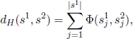
The construction phase iteratively builds a feasible solution, one element at a time. At each iteration, the choice of the element to be added next is determined by ordering all candidate elements (i.e. those that can be added to the solution) in a candidate list C with respect to a greedy criterion. The probabilistic component of a GRASP is characterized by randomly choosing one of the best candidates in the list, but not necessarily the top candidate. The list of best candidates is called the restricted candidate list (RCL). Algorithm 5.1 depicts the pseudo-code of the GRASP for the FFMSP proposed in [FER 13b]. The objective function to be maximized according to [5.17] is denoted by ![]() For each position j ∈ {1, … , m} and for each character c ∈ Σ, Vj(c) is the number of times c appears in position j in any of the strings in Ω. In line 2, the incumbent solution sbest is set to the empty solution with a corresponding objective function value ft(sbest) equal to −∞. The for-loop in lines 3–6 computes
For each position j ∈ {1, … , m} and for each character c ∈ Σ, Vj(c) is the number of times c appears in position j in any of the strings in Ω. In line 2, the incumbent solution sbest is set to the empty solution with a corresponding objective function value ft(sbest) equal to −∞. The for-loop in lines 3–6 computes ![]() and
and ![]() as the minimum and the maximum function value Vj(c) all over characters c ∈ Σ, respectively. Then, until the stopping criterion is no longer met, the while-loop in lines 7–13 computes a GRASP incumbent solution sbest which is returned as output in line 14.
as the minimum and the maximum function value Vj(c) all over characters c ∈ Σ, respectively. Then, until the stopping criterion is no longer met, the while-loop in lines 7–13 computes a GRASP incumbent solution sbest which is returned as output in line 14.
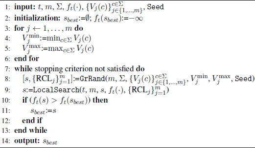
Algorithm 5.2 shows a pseudo-code of the construction procedure that iteratively builds a sequence s = (s1, … , sm) ∈ Σm, selecting one character at time. The greedy function is related to the occurrence of each character in a given position. To define the construction mechanism for the RCL, once ![]() and
and ![]() are known, a cut-off value
are known, a cut-off value ![]() is computed in line 5, where α is a parameter such that 0 ≤ α ≤ 1 (line 4). Then, the RCL is made up of all characters whose greedy function value is less than or equal to μ (line 8). A character is then selected, uniformly at random, from the RCL (line 11).
is computed in line 5, where α is a parameter such that 0 ≤ α ≤ 1 (line 4). Then, the RCL is made up of all characters whose greedy function value is less than or equal to μ (line 8). A character is then selected, uniformly at random, from the RCL (line 11).
Algorithm 5.1. GRASP for the FFMSP
Algorithm 5.2. Function GRRAND of Algorithm 5.1
The basic GRASP local search step consists of investigating all positions j ∈ {1, … , m} and changing the character in position j in the sequence s to another character in RCLj. The current solution is replaced by the first improving neighbor and the search stops after all possible moves have been evaluated and no improving neighbor has been found, returning a locally optimal solution. The worst case computational complexity of the local search procedure is O(n · m · |Σ|). In fact, since the objective function value is at most n, the while-loop in lines 2–14 runs at most n times. Each iteration costs O(m · |Σ|), since for each j = 1, … , m, |RCLj| ≤ |Σ| − 1.
5.4.3.2. The hybrid heuristic evaluation function
The objective function of any instance of the FFMSP is characterized by large plateaus, since there are |Σ|m points in the search space with only n different objective values. To efficiently handle the numerous local maxima, Mousavi et al. [MOU 12a] proposed a new function to be used in the GRASP framework in conjunction with the objective function when evaluating neighbor solutions during the local search phase.
Given a candidate solution s ∈ Σm, the following further definitions and notations are needed:
- – Near(s) = {sj ∈ Ω | dH(s, sj) ≤ t} is the subset of the input strings whose Hamming distance from s is at most t;
- – for each input string sj ∈ Ω, its cost is defined as c(sj, s) = t−dH(s, sj);
- – a L-walk, L ∈
 , 1 ≤ L ≤ m, is a walk of length L in the solution space. A L-walk from s leads to the replacement of s with a solution
  so that
- – given a L-walk from s to a solution s and an input string sj ∈ Ω, then

- – a L-walk from s is random if
 is equally likely to be any solution ŝ where dH (s, ŝ) = L.
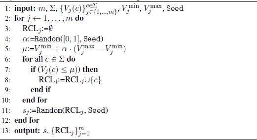
In the case of a random L-walk, Δj is a random variable and PrL(Δj ≤ k), k ∈ ![]() , denotes the probability of Δj ≤ k as a result of a random walk.
, denotes the probability of Δj ≤ k as a result of a random walk.
- – where sj ∈ Near(s) and L = c(sj, s), the potential gain gj(s) of sj with respect to s is defined as follows:
- – where sj ∈ Near(s) and L = c(sj, s):
- - the potential gain gj(s) of sj with respect to s is defined as follows:
- - the Gain-per-Cost GpC(s) of s is defined as the average of the gain per cost of the sequences in Near(s):
- - the potential gain gj(s) of sj with respect to s is defined as follows:
Computing the gain-per-cost of candidate solutions requires knowledge of the probability distribution function of Δk for all possible lengths of random walks and this task has high computational complexity. To reduce the computational effort, Mousavi et al. proposed to approximate all these probability distribution functions with the probability distribution function for a unique random variable Δ corresponding to a random string as a representative of all the strings in Ω. With respect to a random L-walk, Δ is defined as ![]() , where ŝ is a random string (and not an input string) and s and
, where ŝ is a random string (and not an input string) and s and ![]() are the source and destination of the random L-walk, respectively. Once the probability distribution function for the random variable Δ is known, to evaluate candidate solutions based on their likelihood of leading to better solutions, Mousavi et al. define the
are the source and destination of the random L-walk, respectively. Once the probability distribution function for the random variable Δ is known, to evaluate candidate solutions based on their likelihood of leading to better solutions, Mousavi et al. define the ![]() as follows:
as follows:
where s is a candidate solution, and ![]() is the estimated gain of sj, with respect to s, defined as follows:
is the estimated gain of sj, with respect to s, defined as follows:
Then, they define a heuristic function ![]() which takes into account both the objective function
which takes into account both the objective function ![]() and the estimated gain-per-cost function
and the estimated gain-per-cost function ![]()
Given two candidate solutions ![]() function
function ![]() must combin
must combin ![]() and
and ![]() in such a way that:
in such a way that:
if and only if either ![]() and
and ![]() In other words, according to function
In other words, according to function ![]() the candidate solution
the candidate solution ![]() is considered better than ŝ if it corresponds to a better objective function value or the objective function assumes the same value when evaluated in both solutions, but
is considered better than ŝ if it corresponds to a better objective function value or the objective function assumes the same value when evaluated in both solutions, but ![]() has a higher probability of leading to better solutions. Based on proven theoretical results, Mousavi et al. proposed the following heuristic function
has a higher probability of leading to better solutions. Based on proven theoretical results, Mousavi et al. proposed the following heuristic function ![]() where s is a candidate solution:
where s is a candidate solution:
Looking at the results of a few experiments conducted in [MOU 12a], it emerges that use of the hybrid heuristic evaluation function ![]() in place of the objective function
in place of the objective function ![]() in the GRASP local search proposed by Festa [FES 07] results in a reduction in the number of local maxima. Consequently the algorithm’s climb toward better solutions is sped up. On a large set of both real-world and randomly-generated test instances, Ferone et al. [FER 16] conducted a deeper experimental analysis to help determine whether the integration of the hybrid heuristic evaluation function
in the GRASP local search proposed by Festa [FES 07] results in a reduction in the number of local maxima. Consequently the algorithm’s climb toward better solutions is sped up. On a large set of both real-world and randomly-generated test instances, Ferone et al. [FER 16] conducted a deeper experimental analysis to help determine whether the integration of the hybrid heuristic evaluation function ![]() of Mousavi et al. in a GRASP is beneficial. The following two sets of problems were used:
of Mousavi et al. in a GRASP is beneficial. The following two sets of problems were used:
- – Set A: this is the set of benchmarks introduced in [FER 13b], consisting of 600 random instances of different sizes. The number n of input sequences in Ω is {100, 200, 300, 400} and the length m of each of the input sequences is {300, 600, 800}. In all cases, the alphabet consists of four letters, i.e. |Σ| = 4. For each combination of n and m, the set A consists of 100 random instances. The threshold parameter t varies from 0.75 m to 0.85 m.
- – Set B: this set of problems was used in [MOU 12a]. Some instances were randomly generated, while the remaining are real-world instances from biology (Hyaloperonospora parasitica V 6.0 sequence data). In both randomly-generated and real-world instances, the alphabet as four letters, i.e.|Σ| = 4, the number n of input sequences in Ω is {100, 200, 300} and the length m of each of the input sequence ranges from 100 to 1200. Finally, the threshold parameter t varies from 0.75 m to 0.95 m.
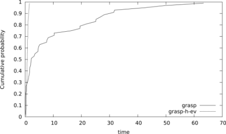
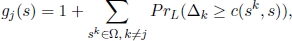
Figure 5.1. Time to target distributions (in seconds) comparing grasp and grasp-h-ev for a random instance where n = 100, m = 600, t = 480, with a target value of  = 0.68 × n
Looking at the results, Ferone et al. concluded that either the two algorithms find the optimal solution or the hybrid GRASP with the Mousavi et al. evaluation function finds better quality results. The further investigation performed by the authors that involves the study of the empirical distributions of the random variable time-to-target-solution-value (TTT-plots) considering the following instances is particulars interesting:
- 1) random instance where n = 100, m = 600, t = 480 and target value = 0.68 × n (Figure 5.1);
- 2) random instance where n = 200, m = 300, t = 255 and target value = 0.025 × n (Figure 5.2);
- 3) real instance where n = 300, m = 1200, t = 1, 020 and target value = 0.22 × n (Figure 5.3).
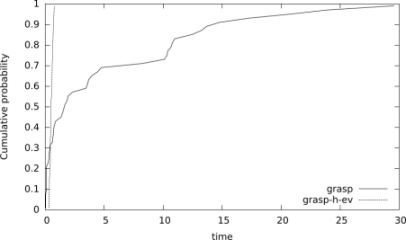
Figure 5.2. Time to target distributions (in seconds) comparing grasp and grasp-h-ev for a random instance where n = 200, m = 300, t = 255, and a target value of = 0.025 × n
Figure 5.3. Time to target distributions (in seconds) comparing grasp and grasp-h-ev for a real instance where n = 300, m = 1200, t = 1020, and a target value of = 0.22 × n
Ferone et al. performed 100 independent runs of each heuristic using 100 different random number generator seeds and recorded the time taken to find a solution at least as good as the target value ![]() . As in [AIE 02], to plot the empirical distribution, a probability
. As in [AIE 02], to plot the empirical distribution, a probability ![]() is associated with the ith sorted running time (ti) and the points zi = (ti, pi), for i = 1, … , 100, are plotted. As shown in Figures 5.1–5.3, we can observe that the relative position of the curves implies that, given any fixed amount of run time, the hybrid GRASP with the Mousavi et al. evaluation function (
is associated with the ith sorted running time (ti) and the points zi = (ti, pi), for i = 1, … , 100, are plotted. As shown in Figures 5.1–5.3, we can observe that the relative position of the curves implies that, given any fixed amount of run time, the hybrid GRASP with the Mousavi et al. evaluation function (grasp-h-ev) has a higher probability of finding a solution with an objective function value at least as good as the target objective function value than pure GRASP (grasp).
5.4.3.3. Path-relinking
Path-relinking is a heuristic proposed by Glover [GLO 96, GLO 00b] in 1996 as an intensification strategy exploring trajectories connecting elite solutions obtained by Tabu search or scatter search [GLO 00a, GLO 97, GLO 00b, RIB 12].
Starting from one or more elite solutions, paths in the solution space leading towards other guiding elite solutions are generated and explored in the search for better solutions. This is accomplished by selecting moves that introduce attributes contained in the guiding solutions. At each iteration, all moves that incorporate attributes of the guiding solution are analyzed and the move that best improves (or least deteriorates) the initial solution is chosen.
Algorithm 5.3 illustrates the pseudo-code of path-relinking for the FFMSP proposed by Ferone et al. in [FER 13b]. It is applied to a pair of sequences (s′ , ŝ). Their common elements are kept constant and the space spanned by this pair of solutions is searched with the objective of finding a better solution. This search is done by exploring a path in the space linking solution s′ to solution ŝ. s′ is called the initial solution and ŝ the guiding solution.
Algorithm 5.3. Path-relinking for the FFMSP
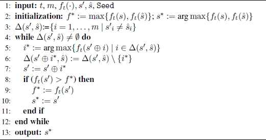
The procedure (line 3) computes the symmetric difference Δ(s′, ŝ) between the two solutions as the set of components for which the two solutions differ:
Note that, ![]() and
and ![]() represents the set of moves needed to reach ŝ from s′, where a move applied to the initial solution s′ consists of selecting a position
represents the set of moves needed to reach ŝ from s′, where a move applied to the initial solution s′ consists of selecting a position ![]() and replacing
and replacing ![]() with ŝi.
with ŝi.
Path-relinking generates a path of solutions ![]() linking s′ and ŝ. The best solution s* in this path is returned by the algorithm (line 13). The path of solutions is computed in the loop in lines 4 through 12. This is achieved by advancing one solution at a time in a greedy manner. At each iteration, the procedure examines all moves i ∈ Δ(s′, ŝ) from the current solution s′ and selects the one which results in the highest cost solution (line 5), i.e. the one which maximizes ft(s′ ⊕ i), where s′ ⊕ i is the solution resulting from applying move i to solution s′. The best move i* is made, producing solution s′ ⊕ i* (line 7). The set of available moves is updated (line 6). If necessary, the best solution s* is updated (lines 8–11). The algorithm stops when Δ(s′ , ŝ) = ∅.
linking s′ and ŝ. The best solution s* in this path is returned by the algorithm (line 13). The path of solutions is computed in the loop in lines 4 through 12. This is achieved by advancing one solution at a time in a greedy manner. At each iteration, the procedure examines all moves i ∈ Δ(s′, ŝ) from the current solution s′ and selects the one which results in the highest cost solution (line 5), i.e. the one which maximizes ft(s′ ⊕ i), where s′ ⊕ i is the solution resulting from applying move i to solution s′. The best move i* is made, producing solution s′ ⊕ i* (line 7). The set of available moves is updated (line 6). If necessary, the best solution s* is updated (lines 8–11). The algorithm stops when Δ(s′ , ŝ) = ∅.
Given two solutions s′ and ŝ, Ferone et al. adopted the following path-relinking strategies:
- – Forward PR: the path emanates from s′ , which is the worst solution between s′ and ŝ (Algorithm 5.3);
- – Backward PR: the path emanates from s′, which is the best solution between s′ and ŝ (Algorithm 5.3);
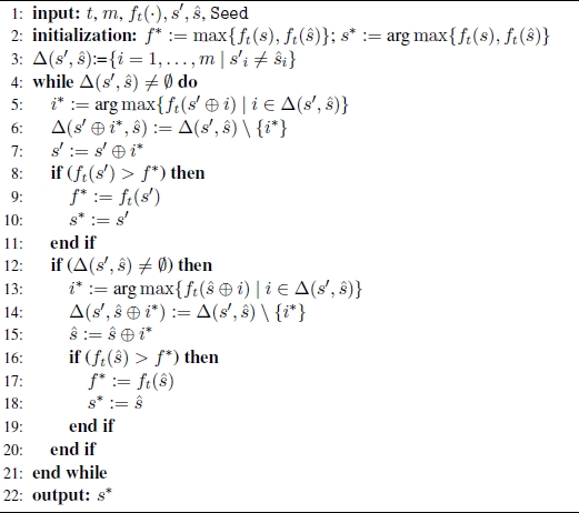
- – Mixed PR: two paths are generated, one emanating from s′ and the other emanating from ŝ. The process stops as soon as an intermediate common solution is met (Algorithm 5.4);
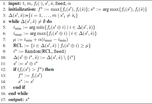
- – Greedy Randomized Adaptive Forward PR: the path emanates from the worst solution between s′ and ŝ. At each iteration a move is made towards an intermediate solution selected at random from among a subset of top-ranked solutions (Algorithm 5.5);
- – Evolutionary PR: a greedy randomized adaptive forward PR is performed at each iteration. At fixed intervals the elite pool is intensified. In fact, at each
EvIterationsiteration, the algorithmEvolutionis invoked (Algorithm 5.6) that performs path-relinking between each pair of current elite set solutions with the aim of eventually improving the current elite set.
Algorithm 5.4. Mixed-Path-relinking for the FFMSP [RIB 07]
5.4.3.4. Hybridizations of GRASP with path-relinking
Ferone et al. [FER 16] integrated a path-relinking intensification procedure in the hybrid GRASP grasp-h-ev described in section 5.4.3.1. The idea behind this integration was to add memory to GRASP and was first proposed in 1999 by Laguna and Martí [LAG 99]. It was followed by several extensions, improvements and successful applications [CAN 01, FES 06, FES 02a, RIB 12].
Algorithm 5.5. (GRAPR) Greedy Randomized Adaptive Path-relinking for FFMSP [FAR 05]
In the hybrid GRASP with path-relinking for the FFMSP, path-relinking is applied at each GRASP iteration to pairs (s, ŝ) of solutions, where s is the locally optimal solution obtained by the GRASP local search and ŝ is randomly chosen from a pool with at most MaxElite high-quality solutions. The pseudo-code for the proposed hybrid GRASP with path-relinking is shown in Algorithm 5.7.
The pool of elite solutions E is empty (line 1) initially and, until E is no longer full, the current GRASP locally optimal solution s is inserted in E. As soon as the pool becomes full (|![]() | =
| = MaxElite), through the Choose-PR-Strategy procedure, the desired strategy for implementing path-relinking is chosen s and solution ŝ are randomly chosen from ![]() . The best solution
. The best solution ![]() found along the relinking trajectory is returned and considered as a candidate to be inserted into the pool. The
found along the relinking trajectory is returned and considered as a candidate to be inserted into the pool. The AddToElite procedure evaluates its insertion into ![]() . If
. If ![]() is better than the best elite solution, then
is better than the best elite solution, then ![]() replaces the worst elite solution. If the candidate is better than the worst elite solution, but not better than the best, it replaces the worst if it is sufficiently different from all elite solutions.
replaces the worst elite solution. If the candidate is better than the worst elite solution, but not better than the best, it replaces the worst if it is sufficiently different from all elite solutions.
Algorithm 5.6. Evolutionary path-relinking for FFMSP [RES 10b, RES 04]
Path-relinking is also applied as post-optimization phase (lines 27–34): at the end of all GRASP iterations, for each different pair of solutions s′, s″ ∈ ![]() , if s′ and s″ are sufficiently different, path-relinking is performed between s′ and s″ by using the same strategy as the intensification phase.
, if s′ and s″ are sufficiently different, path-relinking is performed between s′ and s″ by using the same strategy as the intensification phase.
With the same test instances described in section 5.4.3.2, Ferone et al. comprehensively analyzed of the computational experiments they conducted with the following hybrid GRASPs:
- –
grasp-h-ev, the hybrid GRASP that integrates Mousavi et al.’s evaluation function into the local search; - –
grasp-h-ev_f, the hybrid GRASP approach that adds forward path-relinking to grasp-h-ev; - –
grasp-h-ev_b, the hybrid GRASP that adds backward path-relinking to grasp-h-ev; - –
grasp-h-ev_m, the hybrid GRASP approach that adds Mixed path-relinking to grasp-h-ev; - –
grasp-h-ev_grapr, the hybrid GRASP that adds greedy randomized adaptive forward path-relinking to grasp-h-ev; - –
grasp-h-ev_ev_pr, the hybrid GRASP that adds evolutionary path-relinking to grasp-h-ev.
For the best values to be assigned to several involved parameters, the authors proposed the following settings:
- – setting the maximum number
MaxEliteof elite solutions to 50; - – inserting a candidate solution
 in the elite set
  . If is better than the best elite set solution or is better than the worst elite set solution but not better than the best and its Hamming distance to at least half of the solutions in the elite set is at least 0.75 m, solution replaces the worst solution in the elite set;
 - – in the post-optimization phase, path-relinking is performed between s' and s'' if their Hamming distance is at least 0.75 m.
In terms of average objective function values and standard deviations, Ferone et al. concluded that grasp-h-ev_ev_pr finds slightly better quality solutions compared to the other variants when running for the same number of iterations, while grasp-h-ev_b finds better quality solutions within a fixed running time. To validate the good behavior of the backward strategy, in Figures 5.4 and 5.5, the empirical distributions of the time-to-target-solution-value random variable (TTT-plots) are plot, involving algorithms grasp-h-ev, grasp-h-ev_b and grasp-h-ev_ev_pr without performing path-relinking as post-optimization phase. The plots show that, given any fixed amount of computing time, grasp-h-ev_b has a higher probability than the other algorithms of finding a good quality target solution.
5.4.3.5. Ant colony optimization algorithms
ACO algorithms [DOR 04] are metaheuristics inspired by ant colonies and their shortest path-finding behavior. In 2014, Blum and Festa [BLU 14c] proposed a hybrid between ACO and a mathematical programming solver for the FFMSP. To describe this approach, the following additional notations are needed.
Algorithm 5.7. GRASP+PR for the FFMSP
Algorithm 5.8. CHOOSE-PR-STRATEGY – Function for selection of path-relinking strategy for FFMSP
Given any valid solution s to the FFMSP (i.e. any s of length m over Σ is a valid solution) and a threshold value 0 ≤ t ≤ m, let P s ⊆ Ω be the set defined as follows:
The FFMSP can be equivalently stated as the problem that consists of finding a sequence s* of length m over Σ such that P s* is of maximum size. In other words, the objective function ![]() can be equivalently evaluated as follows:
can be equivalently evaluated as follows:
Moreover, for any given solution s set Qs is defined as the set consisting of all sequences s′ ∈ Ω that have a Hamming distance at least t with respect to s. Formally, the following holds:
Figure 5.4. Time-to-target distributions (in seconds) comparing grasp-h-ev, grasp-h-ev_b and grasp-h-ev_ev_pr on the random instance where n = 100, m = 300, t = 240, and a target value of = 0.73 × n
Figure 5.5. Time-to-target distributions (in seconds) comparing grasp-h-ev, grasp-h-ev_b and grasp-h-ev_ev_pr on the random instance where n = 200, m = 300, t = 240, and a target value of = 0.445 × n
Note that where |P s| < n, set Qs also contains the sequence ŝ ∈ Ω P s that has, among all sequences in Ω P s, the largest Hamming distance with respect to s. To better handle the drawback related to the large plateaus of objective function, the authors proposed slightly modifying the comparison criterion between solutions. Solution s is considered better than solution s (s >lex s ) if and only if the following conditions hold in lexicographical order:
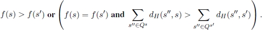
In other words, the comparison between s and s′ is done by considering first the corresponding objective function values and then, as a second criterion, the sum of the Hamming distances of the two solutions from the respective sets Q8 and Q8′ . It is intuitive to assume that the solution for which this sum is greater is somehow closer to a solution with a higher objective function value.
Algorithm 5.9. (Hybrid) ACO for the FFMSP
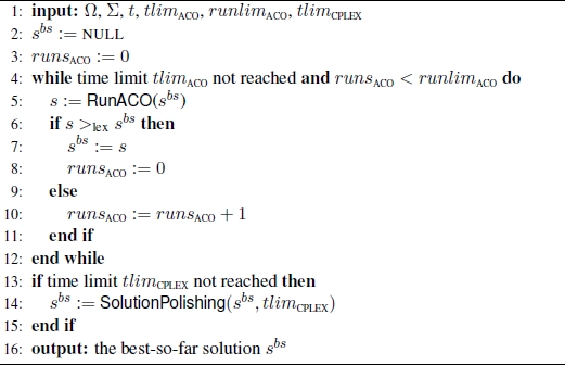
The hybrid ACO (Algorithm 5.9) consists of two phases. After setting the incumbent solution (the best solution found so far) to the empty solution, the first phase (lines 4–12) accomplishes the ACO approach. After this first phase, the algorithm possibly applies a second phase in which hybridization with a mathematical programming solver takes place (lines 13–15). The ACO-phase stops as soon as either a fixed running time limit (tlimACO) has been reached or the number of consecutive unsuccessful iterations (with no improvement of the incumbent solution) has reached a fixed maximum number of iterations (runlimACO).
Algorithm 5.10. RunACO(sbs) function of Algorithm 5.9
The ACO phase is pseudo-coded in Algorithm 5.10. The pheromone model ![]() used consists of a pheromone value τi,cj for each combination of a position i = 1, … , m in a solution sequence and a letter cj ∈ Σ. Moreover, a greedy value, ηi,cj, to each of these combinations is assigned which measures the desirability in reverse proportion letter cj to position i. Intuitively, value ηi,cj should be of assigning to the number of occurrences of letter, cj, at position i in the |Ω| = n input sequences. Formally,
used consists of a pheromone value τi,cj for each combination of a position i = 1, … , m in a solution sequence and a letter cj ∈ Σ. Moreover, a greedy value, ηi,cj, to each of these combinations is assigned which measures the desirability in reverse proportion letter cj to position i. Intuitively, value ηi,cj should be of assigning to the number of occurrences of letter, cj, at position i in the |Ω| = n input sequences. Formally,
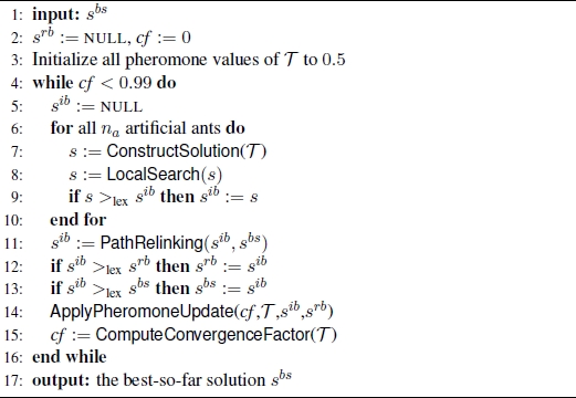
The incumbent solution, sbs, is input as the function which sets all pheromone values of ![]() to 0.5. Then, it proceeds in iterations stopping as soon as the convergence factor value cf is greater than or equal to 0.99. At each iteration of the while-loop (lines 4–16), na = 10 solutions are constructed in the ConstructSolution(
to 0.5. Then, it proceeds in iterations stopping as soon as the convergence factor value cf is greater than or equal to 0.99. At each iteration of the while-loop (lines 4–16), na = 10 solutions are constructed in the ConstructSolution(![]() ) the function on basis of pheromone and greedy information. Starting from each of these solutions, a local search procedure (LocalSearch()) is applied producing a local optimal solution sib to which path-relinking is applied. Solution sib is also referred to as the iteration-best solution. Path-relinking is applied in the PathRelinking(sib, sbs) function. Therefore, sib serves as the initial solution and the best-so-far solution sbs serves as the guiding solution. After updating the best-so-far solution and the so-called restart-best solution, which is the best solution found so far during the current application of RunACO() (if necessary) the pheromone update is performed in function ApplyPheromoneUpdate(cf,
) the function on basis of pheromone and greedy information. Starting from each of these solutions, a local search procedure (LocalSearch()) is applied producing a local optimal solution sib to which path-relinking is applied. Solution sib is also referred to as the iteration-best solution. Path-relinking is applied in the PathRelinking(sib, sbs) function. Therefore, sib serves as the initial solution and the best-so-far solution sbs serves as the guiding solution. After updating the best-so-far solution and the so-called restart-best solution, which is the best solution found so far during the current application of RunACO() (if necessary) the pheromone update is performed in function ApplyPheromoneUpdate(cf, ![]() ,sib,srb). At the end of each iteration, the new convergence factor value cf is computed in function ComputeConvergenceFactor(
,sib,srb). At the end of each iteration, the new convergence factor value cf is computed in function ComputeConvergenceFactor(![]() ).
).
ConstructSolution(T) is the function that in line 7 constructs a solution s on the basis of pheromone and greedy information. It proceeds in m iteration, and at each iteration it chooses the character to be inserted in the ith position of s. For each letter cj ∈ Σ, a probability pi,cj position i will be chosen is calculated as follows:
Then, value z is chosen uniformly at random from [0.5, 1.0]. where z ≤ drate, the letter c ∈ Σ with the largest probability value is chosen for position i. Otherwise, a letter c ∈ Σ is chosen randomly with respect to the probability values. drate is a manually chosen parameter of the algorithm set to 0.8.
The local search and path-relinking procedures are those proposed by Ferone et al. [FER 13b] with solution sib playing the role of initial solution and solution sbs that of the guiding solution.
The algorithm works with the following upper and lower bounds for them pheromone values: τmax = 0.999 and τmin = 0.001. Where pheromone values surpasses one of these limits, the value is set to the corresponding limit. This has the effect that complete convergence of the algorithm is avoided. Solutions sib and srb are used to update the pheromone values. The weight of each solution for the pheromone update is determined as a function of the convergence factor cf and the pheromone values τi,cj are updated as follows:
where
Function Δ(s, cj) evaluates to 1 when character cj is to be found at position i of solution s; otherwise it is given the value 0. Moreover, solution sib has weight κib, while the weight of solution srb is κrb and it is required that κib + κrb = 1. The weights that the authors have chosen are the standard ones shown in Table 5.1.
Table 5.1. Setting of κib and κrb depending on the convergence factor cf
| cf < 0.4 | cf ∈ [0.4, 0.6) | cf ∈ [0.6, 0.8) | cf ≥ 0.8 | |
| κib | 1 | 2/3 | 1/3 | 0 |
| κrb | 0 | 1/3 | 2/3 | 1 |
Finally, ComputeConvergenceFactor(![]() ) function computes the value of the convergence factor as follows:
) function computes the value of the convergence factor as follows:
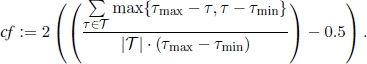
This implies that at the start of function RunACO(sbs), cf has a value of zero. When all pheromone values are either at τmin or at τmax, cf has a value of one. In general, cf moves in [0, 1].
This hybrid ACO (tlimACO = 60s, tlimCPLEX = 90s, runlimACO = 10) has been tested against the same set of benchmarks originally introduced in [FER 13b] and compared with a pure ACO (tlimACO = 90s, tlimCPLEX = 0s, runlimACO = very large integer) and the GRASP hybridized with path-relinking in [FER 13b]. The mathematical model of the problem was solved with IBM ILOG CPLEX V12.1 and the same version of CPLEX was used within the hybrid ACO approach. The (total) computation time limit for each run was set to 90 CPU seconds. The three algorithms are referred to as ACO, HyACO and GRASP+PR, and the results are summarized in Table 5.2. Note that for each combination of n, m and t, the given values are averages of the results of 100 problems. In each case, the best results are shown with a gray background. For the analysis of the results, since the performance of the algorithms significantly changes from one case to another, the three cases resulting from t ∈ {0.75 m, 0.8 m, 0.85 m} are treated separately.
Table 5.2. Numerical results
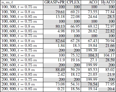
Looking at the results, it is evident that the most interesting case study is represented by those instances characterized by t = 0.85 m. In fact, it turns out that GRASP+PR, as proposed in [FER 13b], is not very effective and that HyACO consistently outperforms the pure ACO approach, which consistently outperforms CPLEX.
5.5. An ILP-based heuristic
Blum and Festa [BLU 16c] proposed a simple two-phase ILP-based heuristic. Since it is based on the ILP model of the problem, it is able to deal with all the four consensus problems described in this chapter.
Given a fixed running time tlimit, for tlimit/2 an ILP solver is used in the first phase to tackle the mixed integer linear problem (MILP) that is obtained by relaxing the xck-variables involved in all four ILP models. After tlimit/2 the ILP solver stops returning the incumbent solution, x′, it found, and that can have some fractional components. In the second phase of the heuristic, the corresponding ILP models are solved in the remaining computation time tlimit/2, with the following additional constraints:
In other words, whenever a variable xck in the best MILP solution-found has a value of 1, this value is fixed for the solution of the ILP model.
Using the same set of benchmarks originally introduced in [FER 13b], this simple heuristic has been compared with the ILP solver applied to the original mathematical models and a simple iterative pure greedy algorithm that builds a solution by adding j = 1, … , m the best ranked character at each iteration according to a greedy criterion that takes into account the number of times each character c ∈ Σ appears in position j in any of the strings in Ω. The (M)ILP solver used in the experiments was IBM ILOG CPLEX V12.1 configured for single-threaded execution. Depending on the problems, two different computation time limits were used: tlimit = 200 seconds and tlimit = 3600 seconds per problem. The different applications of CPLEX and the ILP-based heuristic are named CPLEX-200, CPLEX-3600, HEURISTIC-200 and HEURISTIC-3600.
Table 5.3. Numerical results for the CSP
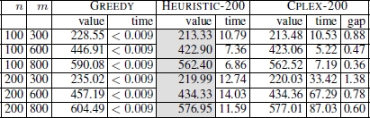
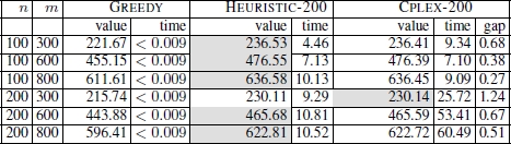
The numerical results for the CSP are shown in Table 5.3. They are presented as averages over 100 instances for each combination of n (the number of input strings) and m (the length of the input strings). For all three algorithms, the table reports the values of the best solutions found (averaged over 100 problem instances) and the computation time at which these solutions were found. In the case of CPLEX-200, the average optimality gap is also provided. The results clearly show that HEURISTIC-200 outperforms both GREEDY and CPLEX-200. Similar conclusions can be drawn in the case of the FSP, for which the results are presented in Table 5.4. Except for one case (n = 200, m = 300) HEURISTIC-200 outperforms both GREEDY and CPLEX-200.
Table 5.4. Numerical results for the FSP
For the CTMSP and the FFMSP, Blum and Festa noticed that the value of t has a significant impact on the hardness of both problems. For the CTMSP, for example, the lower the value of t, the easier it should be for CPLEX to optimally solve the problem. To better understand this relationship, the authors performed the following experiments. CPLEX was applied to each problem – concerning the CTMSP and FFMSP – for each value of t ∈ {0.05m, 0.02m, … , 0.95m}. This was done with a time limit of 3,600 seconds per run. The corresponding optimality gaps (averaged over 100 problems) and the number of instances (out of 100) that were optimally solved are presented in Figure 5.6. The results reveal that, in the case of the CTMSP, the problem becomes difficult for approx. t ≤ 0.72m. In the case of the FFMSP, the problem becomes difficult for approx. t ≥ 0.78m. Therefore, the following values for t were chosen for the final experimental evaluation: t ∈ {0.65m, 0.7m, 0.75m} in the case of the CTMSP, and t ∈ {0.75m, 0.8m, 0.85m} in the case of the FFMSP. The results obtained are reported in Table 5.5 for the CTMSP and in Table 5.6 for the FFMSP.
Table 5.5. Numerical results for the CTMS problem
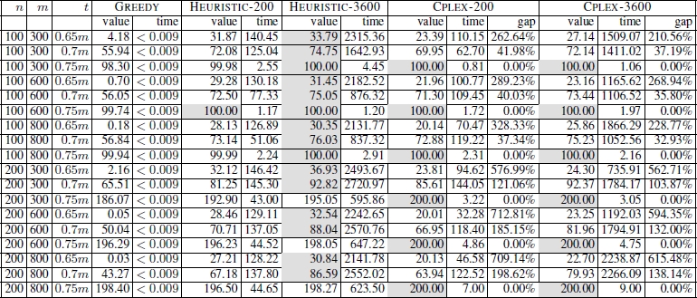
Table 5.6. Results for the FFMS problem
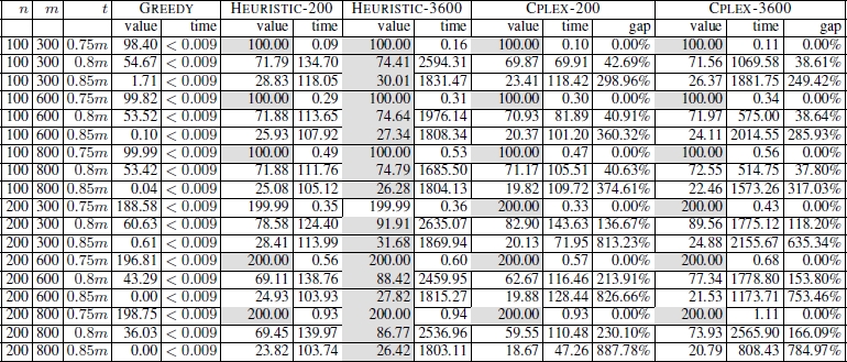
Looking at the numerical results for the CTMSP (for the FFMSP, similar arguments can be made), the following observations can be drawn:
- – both CPLEX and the ILP-based heuristic greatly outperform GREEDY;
- – when the problem is rather easy – that is, for a setting of t = 0.75 m – CPLEX usually has slight advantages over the ILP-based heuristic, especially for instances with a larger number of input strings (n = 200);
- – with growing problem difficulty, the ILP-based heuristic starts to outperform CPLEX; for a setting of t = 0.65 m, the differences in the qualities of the solutions obtained between the ILP-based heuristic and CPLEX are significant.
For the FFMSP, the ILP-based heuristic was also compared with what was then the best state-of-the-art methods, i.e. GRASP+PR proposed by Ferone et al. [FER 13b], the ACO, and the hybrid ACO proposed by Blum and Festa [BLU 14c]. Results of this comparison are presented in Figure 5.7 for all instances where t = 0.8 m and t = 0.85 m. The results show that, for t = 0.8 m, HEURISTIC-3600 is generally outperformed by the other state-of-the-art methods. However, note that when the instance size (in terms of the number of input strings and their length) grows, HEURISTIC-3600 starts to produce better results than the competitors that are outperformed in the harder instances characterized by t = 0.85 m.
5.6. Future work
Following Mousavi et al., one line for future work involves a deeper study of the special characteristics of the objective functions of these consensus problems, whose solution has large plateaus. For problems with this type of objective function, it would be fruitful to apply results from the fitness landscape analysis [PIT 12] , which would greatly help in classifying problems according to their hardness for local search heuristics and meta-heuristics based on local search.
Another line for future research includes the exploration of alternative hybrid approaches obtained by embedding ILP-based method within metaheuristic frameworks.
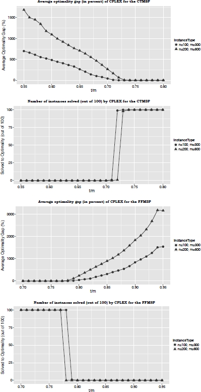
Figure 5.6. Justification for the choice of parameter t for the CTMSP and the FFMSP
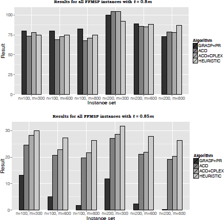
Figure 5.7. Graphical representation of the comparison between HEURISTIC-3600 and the current FFMSP state-of-the-art methods (GRASP+PR, ACO, and ACO+CPLEX) for t = 0.8 m and t = 0.85 m