
1
Introduction
In computer science, a string s is defined as a finite sequence of characters from a finite alphabet Σ. Apart from the alphabet, an important characteristic of a string s is its length which, in this book, will be denoted by |s|. A string is, generally, understood to be a data type i.e. a string is used to represent and store information. For example, words in a specific language are stored in a computer as strings. Even the entire text may be stored by means of strings. Apart from fields such as information and text processing, strings arise in the field of bioinformatics. This is because most of the genetic instructions involved in the growth, development, functioning and reproduction of living organisms are stored in a molecule which is known as deoxyribonucleic acid (DNA) which can be represented in the form of a string in the following way. DNA is a nucleic acid that consists of two biopolymer strands forming a double helix (see Figure 1.1). The two strands of DNA are called polynucleotides as they are composed of simpler elements called nucleotides. Each nucleotide consists of a nitrogen-containing nucleobase as well as deoxyribose and a phosphate group. The four different nucleobases of DNA are cytosine (C), guanine (G), adenine (A) and thymine (T). Each DNA strand is a sequence of nucleotides that are joined to one another by covalent bonds between the sugar of one nucleotide and the phosphate of the next. This results in an alternating sugar–phosphate backbone (see Figure 1.1). Furthermore, hydrogen bonds bind the bases of the two separate polynucleotide strands to make double-stranded DNA. As a result, A can only bind with T and C can only bind with G. Therefore, a DNA molecule can be stored as a string of symbols from Σ = {A, C, T, G} that represent one of the two polynucleotide strands. Similarly, most proteins can be stored as a string of letters from an alphabet of 20 letters, representing the 20 standard amino acids that constitute most proteins.
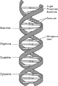
Figure 1.1. DNA double helix (image courtesy of Wikipedia)
As a result, many optimization problems in the field of computational biology are concerned with strings representing, for example, DNA or protein sequences. In this book we will focus particularly on recent works concerning string problems that can be expressed in terms of combinatorial optimization (CO). In early work by Papadimitriou and Steiglitz [PAP 82], a CO problem ![]() is defined by a tuple (
is defined by a tuple (![]() , f), where
, f), where ![]() is a finite set of objects and
is a finite set of objects and ![]() is a function that assigns a non-negative cost value to each of the objects s ∈
is a function that assigns a non-negative cost value to each of the objects s ∈ ![]() . Solving a CO problem
. Solving a CO problem ![]() requires us to find an object s∗ of minimum cost value1. As a classic academic example, consider the well-known traveling salesman problem (TSP). In the case of the TSP, set
requires us to find an object s∗ of minimum cost value1. As a classic academic example, consider the well-known traveling salesman problem (TSP). In the case of the TSP, set ![]() consists of all Hamiltonian cycles in a completely connected, undirected graph with positive edge weights. The objective function value of such a Hamiltonian cycle is the sum of the weights of its edges.
consists of all Hamiltonian cycles in a completely connected, undirected graph with positive edge weights. The objective function value of such a Hamiltonian cycle is the sum of the weights of its edges.
Unfortunately, most CO problems are difficult to optimality solve in practice. In theoretical terms, this is confirmed by corresponding results about non-deterministic (NP)-hardness and non-approximability. Due to the hardness of CO problems, a large variety of algorithmic and mathematical approaches have emerged to tackle these problems in recent decades. The most intuitive classification labels these approaches as either complete/exact or approximate methods. Complete methods guarantee that, for every instance of a CO problem of finite size, there is an optimal solution in bounded time [PAP 82, NEM 88]. However, assuming that P ≠ NP, no algorithm that solves a CO problem classified as being NP-hard in polynomial time exists [GAR 79]. As a result, complete methods, in the worst case, may require an exponential computation time to generate an evincible optimal solution. When faced with large size, the time required for computation may be too high for practical purposes. Thus, research on approximate methods to solve CO problems, also in the bioinformatics field, has enjoyed increasing attention in recent decades. In contrast to complete methods, approximate algorithms produce, not necessarily optimal, solutions in relatively acceptable computation times. Moreover, note that in the context of a combinatorial optimization problem in bioinformatics, finding an optimal solution is often not as important as in other domains. This is due to the fact that often the available data are error prone.
In the following section, we will give a short introduction into some of the most important complete methods, including integer linear programming and dynamic programming. Afterward, some of the most popular approximate methods for combinatorial optimization are reviewed. Finally, the last part of this chapter outlines the string problems considered in this book.
1.1. Complete methods for combinatorial optimization
Many combinatorial optimization problems can be expressed in terms of an integer programming (IP) problem, in a way that involves maximizing or minimizing an objective function of a certain number of decision variables, subject to inequality and/or equality constraints and integrality restrictions on the decision variables.
Formally, we require the following ingredients:
- 1) a n-dimensional vector
 , where each xj, j = 1, 2, … , n, is called a decision variable and x is called the decision vector;
 - 2) m scalar functions
 of the decision vector x;
 - 3) a m-dimensional vector
 , called the right-hand side vector;
 - 4) a scalar function
 of the decision vector x.
With these ingredients, an IP problem can be formulated mathematically as follows:

where ≈ ∈ {≤, =, ≥}. Therefore, the set
is called a feasible set and consists of all those points ![]() that satisfy the m constraints gi(x) ≈ bi, i = 1, 2, … , m. Function z is called the objective function. A feasible point x∗ ∈ X, for which the objective function assumes the minimum (respectively maximum) value i.e. z(x∗) ≤ z(x) (respectively z(x∗) ≥ z(x)) for all x ∈ X is called an optimal solution for (IP).
that satisfy the m constraints gi(x) ≈ bi, i = 1, 2, … , m. Function z is called the objective function. A feasible point x∗ ∈ X, for which the objective function assumes the minimum (respectively maximum) value i.e. z(x∗) ≤ z(x) (respectively z(x∗) ≥ z(x)) for all x ∈ X is called an optimal solution for (IP).
In the special case where ![]() is a finite set, the (IP) problem is a CO problem. The optimization problems in the field of computational biology described in this book are concerned with strings and can be classified as CO problems. Most of them have a binary nature, i.e. a feasible solution to any of these problems is a n-dimensional vector x ∈ {0, 1}n, where for each xi it is necessary to choose between two possible choices. Classical binary CO problems are, for example, the 0/1 knapsack problem, assignment and matching problems, set covering, set packing and set partitioning problems [NEM 88, PAP 82].
is a finite set, the (IP) problem is a CO problem. The optimization problems in the field of computational biology described in this book are concerned with strings and can be classified as CO problems. Most of them have a binary nature, i.e. a feasible solution to any of these problems is a n-dimensional vector x ∈ {0, 1}n, where for each xi it is necessary to choose between two possible choices. Classical binary CO problems are, for example, the 0/1 knapsack problem, assignment and matching problems, set covering, set packing and set partitioning problems [NEM 88, PAP 82].
In what follows, unless explicitly noted, we will refer to a general integer linear programming (ILP) problem in standard form:
where ![]() is the matrix of the technological coefficients aij, i = 1, 2, … , m, j = 1, 2, … , n,
is the matrix of the technological coefficients aij, i = 1, 2, … , m, j = 1, 2, … , n, ![]() and
and ![]() are the m-dimensional array of the constant terms and the n-dimensional array of the objective function coefficients, respectively. Finally,
are the m-dimensional array of the constant terms and the n-dimensional array of the objective function coefficients, respectively. Finally, ![]() is the n-dimensional array of the decision variables, each being non-negative and integer. ILP is linear since both the objective function [1.1] and the m equality constraints [1.2] are linear in the decision variables x1, … , xn.
is the n-dimensional array of the decision variables, each being non-negative and integer. ILP is linear since both the objective function [1.1] and the m equality constraints [1.2] are linear in the decision variables x1, … , xn.
Note that the integer constraints [1.3] define a lattice of points in ![]() n, some of them belonging to the feasible set X of ILP. Formally,
n, some of them belonging to the feasible set X of ILP. Formally, ![]() , where
, where ![]() (Figure 1.2).
(Figure 1.2).
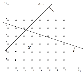
Figure 1.2. Graphical representation of the feasible region X of a generic ILP problem:  , where
Many CO problems are computationally intractable. Moreover, in contrast to linear programming problems that may be solved efficiently, for example by the simplex method, there is no single method capable of solving all of them efficiently. Since many of them exhibit special properties, because they are defined on networks with a special topology or because they are characterized by a special cost structure, the scientific community has historically lavished its efforts on the design and development of ad hoc techniques for specific problems. The remainder of this section is devoted to the description of mathematical programming methods and to dynamic programming.
1.1.1. Linear programming relaxation
A simple way to approximately solving an ILP using mathematical programming techniques is as follows:
a) Relax the integer constraints [1.3], obtaining the following continuous linear programming problem in the standard form:
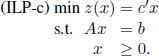
ILP-c is called the linear programming relaxation of ILP. It is the problem that arises by the replacement of the integer constraints [1.3] by weaker constraints that state that each variable xj may assume any non-negative real value. As already mentioned, ILP-c can be solved by applying, for example, the simplex method [NEM 88]. Let x∗ and ![]() be the optimal solution and the optimal objective function value for ILP-c, respectively. Similarly, let
be the optimal solution and the optimal objective function value for ILP-c, respectively. Similarly, let ![]() and
and ![]() be the optimal solution and the optimal objective function value for ILP, respectively.
be the optimal solution and the optimal objective function value for ILP, respectively.
Note that since X ⊂ P, we have:
therefore, ![]() is a lower bound for
is a lower bound for ![]() .
.
b) If ![]() , then x∗ is also an optimal solution for ILP, i.e.
, then x∗ is also an optimal solution for ILP, i.e.
The procedure described above generally results in failure, as the optimal solution x∗ to the linear programming relaxation typically does not have all integer components, except for in special cases such as problems whose formulation is characterized by a totally unimodular matrix A (see the transportation problem, the assignment problem and shortest path problems with non-negative arc lengths). Furthermore, it is wrong to try to obtain a solution xI for ILP by rounding all non-integer components of x∗, because it may lead to infeasible solutions, as shown in Example 1.1 below.
The corresponding feasible set X is depicted in Figure 1.3. Optimal solutions of its linear relaxation are all points ![]() , with
, with ![]() and
and ![]() . Therefore,
. Therefore, ![]() . Moreover,
. Moreover, ![]() , since either xI = (0, 2) or xI = (1, 2).
, since either xI = (0, 2) or xI = (1, 2).
Summarizing, the possible relations between ILP and its linear programming relaxation ILP-c are listed below and X∗ and P∗ denote the set of optimal solutions for ILP and ILP-c, respectively:
- 1)

- 2)
 (not possible in the case of combinatorial optimization problems);
 - 3)
 (lower bound);
 - 4)
 and
and
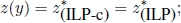
- 5) X = ∅, but P∗ = ∅, as for the problem described in Example 1.1, whose feasible set is depicted in Figure 1.3;
- 6) X = ∅, but
 (not possible in the case of combinatorial optimization problems), as for the following problem, whose feasible set is shown in Figure 1.4:
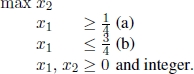
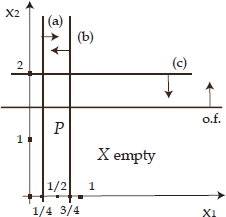
Figure 1.3. Feasible set of the problem described in Example 1.1.  , with
  and
and  . Furthermore,
  , since either xI = (0, 2) or xI = (1, 2)
Even if it almost always leads to failure while finding an optimal solution to ILP, linear programming relaxation is very useful in the context of many exact methods, as the lower bound that it provides avoids unnecessary explorations of portions of the feasible set X. This is the case with branch and bound (B&B) algorithms, as explained in section 1.1.2.1. Furthermore, linear programming relaxation is a standard technique for designing approximation algorithms for hard optimization problems [HOC 96, VAZ 01, WIL 11].
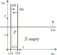
Figure 1.4. Feasible set of the problem described in point (6) below Example 1.1: X = Ø, but 
1.1.2. Cutting plane techniques
Historically, cutting plane techniques were the first algorithms developed for ILP that could be proved to converge in a finite number of steps. A cutting plane algorithm iteratively finds an optimal solution x∗ following linear programming relaxation ILP-c. If x∗ has at least one fractional component, a constraint satisfied by all integer solutions belonging to P, but not satisfied by x∗, is identified. This constraint, which is violated by x∗ and is added to the mathematical formulation of ILP-c, is called a cut. Formally, given x∗ ∈ P, a ∈ ![]() n and b ∈
n and b ∈ ![]() , the constraint a′x ≤ b is a cut if the following two conditions hold:
, the constraint a′x ≤ b is a cut if the following two conditions hold:
- 1)
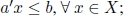
- 2) a′x* > b.
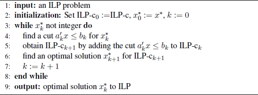
Any cutting plane algorithm proceeds in iterations, as shown in Algorithm 1.1. Different cutting plane algorithms differ from each other in the method they adopt to identify the cut to be added to the current linear programming formulation ILP-ck at each iteration. Since the number of iterations performed corresponds to the number of cuts needed, it is intuitive that stronger cuts imply fewer iterations. Unfortunately, most state-of-the-art cutting plane techniques can cut only small portions of P.
Algorithm 1.1. General Cutting Plane Technique
A feasible solution x ∈ ![]() n of a system Ax = b of equality constraints, A ∈
n of a system Ax = b of equality constraints, A ∈ ![]() m×n and b ∈
m×n and b ∈ ![]() m, is a basic solution if the n components of x can be partitioned into m non-negative basic variables and n − m non-basic variables in a way such that the m columns of A, corresponding to the basic variables, form a non-singular submatrix B (basis matrix), and the value of each non-basic variable is 0. In 1958, Gomory [GOM 58] proposed the most famous and well-known cutting plane method, whose basic idea is to exploit important information related to the m×m non-singular submatrix B of A corresponding to the m currently basic variables in the optimal continuous solution x∗.
m, is a basic solution if the n components of x can be partitioned into m non-negative basic variables and n − m non-basic variables in a way such that the m columns of A, corresponding to the basic variables, form a non-singular submatrix B (basis matrix), and the value of each non-basic variable is 0. In 1958, Gomory [GOM 58] proposed the most famous and well-known cutting plane method, whose basic idea is to exploit important information related to the m×m non-singular submatrix B of A corresponding to the m currently basic variables in the optimal continuous solution x∗.
Let us consider a generic iteration k of Gomory’s algorithm. Suppose that the optimal continuous solution ![]() has at least one fractional component. Let xh be such a variable. Clearly, xh must be a basic variable and let us suppose it is carried in the tth row of the optimal table. We can observe that the equation associated with the tth row of the optimal table can be stated as follows:
has at least one fractional component. Let xh be such a variable. Clearly, xh must be a basic variable and let us suppose it is carried in the tth row of the optimal table. We can observe that the equation associated with the tth row of the optimal table can be stated as follows:
where:
- – N is the set of non-basic variables;
- – ātj, j ∈ N are the elements of the tth row of the optimal table corresponding to the columns of the non-basic variables;
- –
 is a fractional constant, by hypothesis.
Since xj ≥ 0, for all j = 1, 2, … , n, we have:
Moreover, since xj must assume an integer value, the following inequality holds:
The tth row of the optimal table is referred to as the row generating the cut and inequality [1.4] is the cut that Gomory’s algorithm uses at each iteration, until it is not obtained in an optimal continuous solution ![]() . It can easily be proved that the cut [1.4] is still satisfied by all feasible integer solution, but violated by
. It can easily be proved that the cut [1.4] is still satisfied by all feasible integer solution, but violated by ![]() , since the current value of the hth component of
, since the current value of the hth component of ![]() is
is ![]() , the components of
, the components of ![]() corresponding to the non-basic variables are zero, and
corresponding to the non-basic variables are zero, and ![]() .
.
1.1.2.1. Branch and Bound
An alternative exact approach is B&B, which is an implicit enumeration technique because it can prove the optimality of a solution without explicitly visiting all valid solutions when it finishes. Almost always outperforming the cutting plane approach, it is a divide and conquer framework that addresses ILP by dividing it into a certain number of subproblems, which are “simpler” because they are smaller in size.
Given the following ILP:
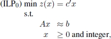
with feasible set X0 and optimal objective function value given by:
we obtain ILP0 B&B partitions in a certain number of subproblems ILP1, … , ILPn0, whose totality represents ILP0. Such a partition is obtained by partitioning X0 into the subsets X1, … , Xn0 such that:
- – for i = 1, … , n0, Xi is the feasible set of subproblem ILPi;
- – for i = 1, … , n0,
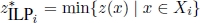 is the optimal objective function value of subproblem ILPi;
 - –
 .
.
Note that, since any feasible solution of ILP0 is feasible for at least one subproblem among ILP1, … , ILPn0, it clearly results that:
Therefore, ILP0 is solved by solving ILP1, … , ILPn0, i.e. for each ILPi, i = 1, … , n0. One of the three options given below will hold true:
- – an optimal solution to ILPi is found; or
- – it can be proved that ILPi is unfeasible (Xi = ∅); or
- – it can be proved that an optimal solution to ILPi is not better than a known feasible solution to ILP0 (if any).
Each ILPi subproblem, i = 1, … , n0, has the same characteristics and properties as ILP0. Hence, the procedure described above can be applied to solve it, i.e. its feasible set Xi is partitioned and so on.
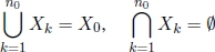
The whole process is usually represented dynamically by means of a decision tree, also called a branching tree (see Figure 1.5), where:
- – the choice of the term branching refers to the partitioning operation of Xi sets;
- – the choice of the classical terms used in graph and tree theory include:
- - root node (corresponding to the original problem ILP0),
- - father and children nodes,
- - leaves, each corresponding to some ILPi subproblem, i > 0, still to be investigated.
Figure 1.5. Branch and bound branching tree
It is easily understandable and intuitive that the criterion adopted to fragment every ILPi (sub)problem, i = 0, 1, … , n0, has a huge impact on the computational performance of a B&B algorithm. In the literature, several different criteria have been proposed to perform this task, each closely connected to some specific procedure, called a relaxation technique. Among the well-known relaxation techniques, those that ought to be mentioned are:
- – linear programming relaxation;
- – relaxation by elimination;
- – surrogate relaxation;
- – Lagrangian relaxation;
- – relaxation by decomposition.
The most frequently applied relaxation technique is linear programming relaxation. To understand the idea underlying this technique, let us consider ILP0 with feasible set X0 depicted in Figure 1.6. The optimal solution to its linear programming relaxation (with feasible set P0) is ![]() , with
, with ![]() . Clearly, in the optimal integer solution it must be either x1 ≤ 1 or x1 ≥ 2. Therefore, one can proceed by separately adding to the original integer formulation of ILP0 the constraints x1 ≤ 1 and x1 ≥ 2, respectively. By adding constraint x1 ≤ 1, the subproblem ILP x1≤1 is generated, with the optimal solution
. Clearly, in the optimal integer solution it must be either x1 ≤ 1 or x1 ≥ 2. Therefore, one can proceed by separately adding to the original integer formulation of ILP0 the constraints x1 ≤ 1 and x1 ≥ 2, respectively. By adding constraint x1 ≤ 1, the subproblem ILP x1≤1 is generated, with the optimal solution ![]() . Similarly, by adding constraint x1 ≥ 2, the subproblem ILP x1≥2 is generated, with the optimal solution
. Similarly, by adding constraint x1 ≥ 2, the subproblem ILP x1≥2 is generated, with the optimal solution ![]() . In this way, ILP0 is partitioned into the two subproblems ILP x1≤1 and ILP x1≥2, whose feasible sets (see Figure 1.7) are X1 and X2 such that X1 ∪ X2 = X0 and
. In this way, ILP0 is partitioned into the two subproblems ILP x1≤1 and ILP x1≥2, whose feasible sets (see Figure 1.7) are X1 and X2 such that X1 ∪ X2 = X0 and ![]() . An optimal solution to ILP0 is obtained with the best solution between
. An optimal solution to ILP0 is obtained with the best solution between ![]() and
and ![]() .
.
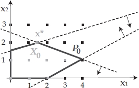
Figure 1.6. B&B scenario
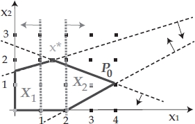
Figure 1.7. B&B partitioning (branching)
More generally, given ILP0, one needs to solve its linear programming relaxation:
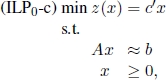
with feasible set P0. Let ![]() be an optimal solution to ILP0-c. If all components of
be an optimal solution to ILP0-c. If all components of ![]() are integer, then
are integer, then ![]() is an optimal solution to ILP0. Otherwise, (see Figure 1.8) a fractional component
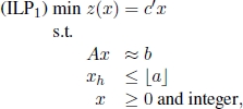
is an optimal solution to ILP0. Otherwise, (see Figure 1.8) a fractional component ![]() is chosen and the following two subproblems are identified:
is chosen and the following two subproblems are identified:
and
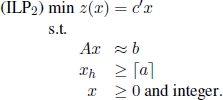
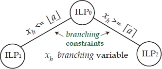
Figure 1.8. Branching: 
Identifying subproblems ILP1 and ILP2 starting from ILP0 corresponds to performing a branching operation. Variable xh is called the branching variable. Subproblems ILP1 and ILP2 are children of ILP0 as they are obtained by adding the branching constraints ![]() and
and ![]() , respectively to the formulation of ILP0.
, respectively to the formulation of ILP0.
Since ILP1 and ILP2 are still integer problems, they are approached with the same procedure, i.e. for each of them its linear relaxation is optimally solved and, if necessary, further branching operations are performed. Proceeding in this way, we obtain a succession of hierarchical subproblems that are more constrained and hence easier to solve. As already underlined, the whole process is represented dynamically by means of a decision tree, also called a branching tree, whose root node corresponds to the original problem, ILP0. Any child node corresponds to the subproblem obtained by adding a branching constraint to the formulation of the problem corresponding to its father node.
Generally speaking, the constraints of any subproblem ILPt corresponding to node t in the branching tree are the following ones:
- 1) the constraints of the original problem, ILP0;
- 2) the branching constraints that label the unique path in the branching tree from the root node to node t (node t “inherits” the constraints of its ancestors).
In principle, the branching tree could represent all possible branching operations and, therefore, be a complete decision tree that enumerates all feasible solutions to ILP0. Nevertheless, as explained briefly, thanks to the bounding criterion, entire portions of the feasible region X0 that do not contain the optimal solution are not explored or, in other words, a certain number of feasible solutions are not generated, since they are not optimal.
Let us suppose that the B&B algorithm is evaluating subproblem ILPt and let xopt be the best current solution (incumbent solution) to ILP0 (i.e. xopt is an optimal solution to at least one subproblem, ILPk, k > 0 and ![]() among those subproblems already investigated). Let zopt = z(xopt), where initially zopt := +∞ and xopt := ∅.
among those subproblems already investigated). Let zopt = z(xopt), where initially zopt := +∞ and xopt := ∅.
Recalling the possible relations existing between a linear integer program and its linear programming relaxation described in section 1.1.1, it is useless to operate a branch from ILPt if any of the following three conditions holds:
- 1) The linear programming relaxation ILPt-c is infeasible (hence, ILPt is infeasible as well). This happens when the constraints of the original problem, ILP0, and the branching constraints from the root of the branching tree to node t are inconsistent;
- 2) The optimal solution to linear programming relaxation ILPt-c is integer. In this case, if necessary, xopt and zopt are updated.
- 3) The optimal solution to linear programming relaxation ILPt-c is not integer, but:
In the latter case, it is clearly useless to keep partitioning Xt. This is because none of the feasible integer solutions are better than the incumbent solution xopt, since it always holds that ![]() . Inequality [1.5] is called the bounding criterion.
. Inequality [1.5] is called the bounding criterion.
1.1.2.2. Choice of branching variable
Suppose that the B&B algorithm is investigating subproblem ILPt and that a branching operation must be performed because none of the three conditions listed above is verified. Let ![]() be an optimal solution to ILPt-c and suppose that it has at least two fractional components, i.e.
be an optimal solution to ILPt-c and suppose that it has at least two fractional components, i.e.
The most commonly used criteria adopted to choose the branching variable xh are as follows:
- 1) h is randomly selected from set F;
- 2)
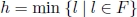 (h is the minimum index in F);
 - 3)
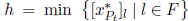 (h is the index in F corresponding to the minimum fractional value).
1.1.2.3. Generation/exploration of the branching tree
A further issue that still remains to be determined is the criterion for generating/exploring the branching tree. At each iteration, a B&B algorithm maintains and updates a list Q of live nodes in the branching tree, i.e. a list of the current leaves that correspond to the active subproblems:
Two main techniques are adopted to decide the next subproblem in Q to be investigated:
- – Depth first: recursively, starting from the last generated node t corresponding to subproblem ILPt whose feasible region Xt must be partitioned, its left child is generated/explored, until node k corresponding to subproblem ILPk is generated from which no branch is needed. In the latter case, backtracking is performed to the first active node j < k that has already been generated. Usually, set Q is implemented as a stack and the algorithm stops as soon as Q = ∅, i.e. when a backtrack to the root node must be performed.
This technique has the advantages of being relatively easier to implement and of keeping the number of active nodes low. Moreover, it produces feasible solutions rapidly, which means that good approximate solutions are obtained even when stopped rather early (e.g. in the case of the running time limit being reached). On the other hand, deep backtracks must often be performed.
- – Best bound first: at each iteration, the next active node to be considered is the node associated with subproblem ILPt corresponding to the linear programming relaxation with the current best objective function value, i.e.
The algorithm stops as soon as Q = ∅. This technique has the advantage of generating a small number of nodes, but rarely goes to very deep levels in the branching tree.
1.1.3. General-purpose ILP solvers
The techniques described in the previous section, among others, are implemented as components of general-purpose ILP solvers that may be applied to any ILP. Examples of such ILP solvers include IBM ILOG CPLEX [IBM 16], Gurobi [GUR 15] and SCIP [ACH 09]. The advantage of these solvers is that they are implemented in an incredibly efficient way and they incorporate all cutting-edge technologies. However, for some CO problems it might be more efficient to develop a specific B&B algorithm, for example.
1.1.4. Dynamic programming
Dynamic programming is an algorithmic framework for solving CO problems. Similar to any divide and conquer scheme, it is based on the principle that it is possible to define an optimal solution to the original problem in terms of some combination of optimal solutions to its subproblems. Nevertheless, in contrast to the divide and conquer strategy, dynamic programming does not partition the problem into disjointed subproblems. It applies when the subproblems overlap, i.e. when subproblems share themselves. More formally, two subproblems (ILPh) and (ILPk) overlap if they can be divided into the following subproblems:
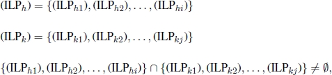
where (ILPh) and (ILPk) share at least one subproblem.
A CO ILP problem can be solved by the application of a dynamic programming algorithm if it exhibits the following two fundamental characteristics:
- 1) ILP exhibits an optimal substructure, i.e. an optimal solution to ILP contains optimal solutions to its subproblems. This characteristic guarantees there is a formula that correctly expresses an optimal solution to ILP as combination of optimal solutions to its subproblems.
- 2) ILP must be divisible into overlapping subproblems. From a computational point of view, any dynamic programming algorithm takes advantage of this characteristic. It solves each subproblem, ILPl, only once and stores the optimal solution in a suitable data structure, typically a table. Afterwards, whenever the optimal solution to ILPl is needed, this optimal solution is looked up in the data structure using constant time per lookup.
When designing a dynamic programming algorithm for a CO ILP problem, the following three steps need to be taken:
- 1) Verify that ILP exhibits an optimal substructure.
- 2) Recursively define the optimal objective function value as combination of the optimal objective function value of the subproblems (recurrence equation). In this step, it is essential to identify the elementary subproblems, which are those subproblems that are not divisible into further subproblems and thus are immediately solvable (initial conditions).
- 3) Write an algorithm based on the recurrence equation and initial conditions stated in step 2.
1.2. Approximate methods: metaheuristics
In contrast to complete (or exact) techniques as outlined in the previous section, metaheuristics [BLU 03, GEN 10a] are approximate methods for solving optimization problems. They were introduced in order to provide high-quality solutions using a moderate amount of computational resources such as computation time and memory. Metaheuristics are often described as “generally applicable recipes” for solving optimization problems. The inspiration for specific metaheuristics are, taken from natural processes, such as the annealing of glass or metal that give rise to a metaheuristic known as simulated annealing (see section 1.2.5) and the shortest path-finding behavior of natural ant colonies that inspired the ant colony optimization (ACO) metaheuristic (see section 1.2.1). Many ideas originate from the way of visualizing the search space of continuous and CO problems in terms of a landscape with hills and valleys. When a maximization problem is considered, the task is then to find the highest valley in the search landscape. The general idea of a local search, for example, is to start the search process at some point in the search landscape and then move uphill until the peak of a mountain is reached. In analogy, an alternative expression for a search procedure based on a local search is hill-climber. Several metaheuristics are extensions of a simple local search, equipped with strategies for moving from the current hill to other (possibly neighboring) hills in the search landscape. In any case, during the last 40–50 years, metaheuristics have gained a strong reputation for tackling optimization problems to which complete methods cannot be applied – for example, due to the size of the problem considered – and for problems for which simple greedy heuristics do not provide solutions of sufficient quality.
As mentioned above, several metaheuristics are extensions of a simple local search. To formally define a local search method, the notion of a so-called neighborhood must be introduced. Given a CO problem (![]() , f), where
, f), where ![]() is the search space – that is, the set of all valid solutions to the problem – and
is the search space – that is, the set of all valid solutions to the problem – and ![]() is the objective function that assigns a positive cost value to each valid solution S ∈
is the objective function that assigns a positive cost value to each valid solution S ∈ ![]() , a neighborhood is defined as a function,
, a neighborhood is defined as a function, ![]() 2
2![]() . In other words, a neighborhood assigns to each solution S ∈
. In other words, a neighborhood assigns to each solution S ∈ ![]() a subset N(S) ⊆
a subset N(S) ⊆ ![]() which is called the neighborhood of S. Any solution s such that f(S) ≤ f(S′) for all S′ ∈ N(S) is called a local minimum with respect to N. Moreover, a solution S∗ such that f(S∗) ≤ f(S′) for all S′ ∈
which is called the neighborhood of S. Any solution s such that f(S) ≤ f(S′) for all S′ ∈ N(S) is called a local minimum with respect to N. Moreover, a solution S∗ such that f(S∗) ≤ f(S′) for all S′ ∈ ![]() is called a global minimum. Note that any global minimum is a local minimum with respect to any neighborhood at the same time.
is called a global minimum. Note that any global minimum is a local minimum with respect to any neighborhood at the same time.
Algorithm 1.2. Local search
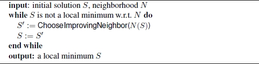
Given a neighborhood N, a simple local search method can be defined as follows; see also Algorithm 1.2. First, an initial solution S must be generated. This may be done randomly, or by means of a greedy heuristic. Then, at each step a solution S′ ∈ N(S) is chosen in function ChooseImproving Neighbor (N(S)) such that f(S′) < f(S). Solution S is then replaced by S′ and the algorithm proceeds to the next iterations. There are at least two standard ways of implementing function ChooseImproving Neighbor (N(S)). In the first one – henceforth, referred to as best-improvement local search – S′ is chosen as follows:
The second standard way of implementing this function is firstimprovement local search. In first-improvement local search, the solutions to N(S) are ordered in some way. They are then examined in the order they are produced and the first solution that has a lower objective function value than S (if any) is returned.
In general, the performance of a local search method depends firmly on the choice of the neighborhood N. It is also interesting to note that a local search algorithm partitions the search space into so-called basins of attraction of local minima. Hereby, the basin of attraction B(S) of a local minimum S ∈ ![]() is a subset of the search space, i.e. B(S) ⊆
is a subset of the search space, i.e. B(S) ⊆ ![]() . In particular, when starting the local search under consideration from any solution S′ ∈ B(S), the local minimum at which the local search method stops is S. In relation to constructive heuristics, it can be stated that constructive heuristics are often faster than local search methods, yet they frequently return solutions of inferior quality.
. In particular, when starting the local search under consideration from any solution S′ ∈ B(S), the local minimum at which the local search method stops is S. In relation to constructive heuristics, it can be stated that constructive heuristics are often faster than local search methods, yet they frequently return solutions of inferior quality.
In the following section, we will describe some important metaheuristics. With the exception of evolutionary algorithms (see section 1.2.2), all these metaheuristics are either extensions of constructive heuristics or of a local search. The order in which the metaheuristics are described is alphabetical.
1.2.1. Ant colony optimization
ACO [DOR 04] is a metaheuristic which was inspired by the observation of the shortest-path finding behavior of natural ant colonies. From a technical perspective, ACO algorithms are extensions of constructive heuristics. Valid solutions to the problem tackled are assembled as subsets of the complete set C of solution components. In the case of the traveling salesman problem (TSP), for example, C may be defined as the set of all edges of the input graph. At each iteration of the algorithm, a set of na solutions are probabilistically constructed based on greedy information and on so-called pheromone information. In a standard case, for each solution with components c ∈ C, the algorithm considers a pheromone value τc ∈ ![]() , where
, where ![]() is the set of all pheromone values. Given a partial solution, Sp ⊆ C, the next component c′ ∈ C to be added to Sp is chosen based on its pheromone value τc′ and the value η(c′) of a greedy function η(·). Set
is the set of all pheromone values. Given a partial solution, Sp ⊆ C, the next component c′ ∈ C to be added to Sp is chosen based on its pheromone value τc′ and the value η(c′) of a greedy function η(·). Set ![]() is commonly called the pheromone model, which is one of the central components of any ACO algorithm. The solution construction mechanism together with the pheromone model and the greedy information define a probability distribution over the search space. This probability distribution is updated at each iteration (after having constructed na solutions) by increasing the pheromone value of solution components that appear in good solutions constructed in this iteration or in previous iterations.
is commonly called the pheromone model, which is one of the central components of any ACO algorithm. The solution construction mechanism together with the pheromone model and the greedy information define a probability distribution over the search space. This probability distribution is updated at each iteration (after having constructed na solutions) by increasing the pheromone value of solution components that appear in good solutions constructed in this iteration or in previous iterations.
In summary, ACO algorithms attempt to solve CO problems by iterating the following two steps:
- – candidate solutions are constructed by making use of a mechanism for constructing solutions, a pheromone model and greedy information;
- – candidate solutions are used to update the pheromone values in a way that is deemed to bias future sampling toward high-quality solutions.
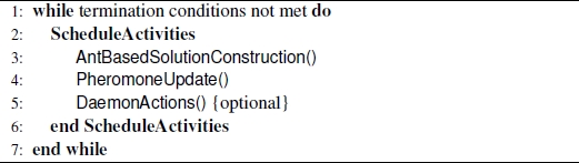
In other words, the pheromone update aims to lead the search towards regions of the search space containing high-quality solutions. The reinforcement of solution components depending on the quality of solutions in which they appear is an important ingredient of ACO algorithms. By doing this, we implicitly assume that good solutions consist of good solution components. In fact, it has been shown that learning which components contribute to good solutions can – in many cases – help to assemble them into better solutions. A high-level framework of an ACO algorithm is shown in Algorithm 1.3. Daemon actions (see line 5 of Algorithm 1.3) mainly refer to the possible application of local search to solutions constructed in the AntBasedSolutionConstruction() function.
A multitude of different ACO variants have been proposed over the years. Among the ones with the best performance are (1) MAX–MIN Ant System (MMAS) [STÜ 00] and (2) Ant Colony System (ACS) [DOR 97]. For more comprehensive information, we refer the interested reader to [DOR 10].
Algorithm 1.3. Ant colony optimization (ACO)
1.2.2. Evolutionary algorithms
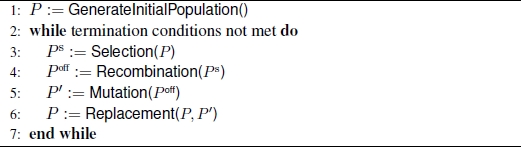
Evolutionary algorithms (EAs) [BÄC 97] are inspired by the principles of natural evolution, i.e. by nature’s capability to evolve living beings to keep them well adapted to their environment. At each iteration, an EA maintains a population P of individuals. Generally, individuals are valid solutions to the problem tackled. However, EAs sometimes also permit infeasible solutions or even partial solutions. Just as in natural evolution, the driving force in EAs is the selection of individuals based on their fitness, which is – in the context of combinatorial optimization problems – usually a measure based on the objective function. Selection takes place in two different operators of an EA. First, selection is used at each iteration to choose parents for one or more reproduction operators in order to generate a set, Poff, of offspring. Second, selection takes place when the individuals in the population of the next iteration are chosen from the current population P and the offspring generated in the current iteration. In both operations, individuals with higher fitness have a higher probability of being chosen. In natural evolution this principle is known as survival of the fittest. Note that reproduction operations, such as crossover, often preserve the solution components that are present in the parents. EAs generally also make use of mutation or modification operators that cause either random changes or heuristically-guided changes in an individual. This process described above is pseudo-coded in Algorithm 1.4.
A variety of different EAs have been proposed over the last decades. To mention all of them is out of the scope of this short introduction. However, three major lines of EAs were independently developed early on. These are evolutionary programming (EP) [FOG 62, FOG 66], evolutionary strategies (ESs) [REC 73] and genetic algorithms (GAs) [HOL 75, GOL 89]. EP, for example, was originally proposed to operate on discrete representations of finite state machines. However, most of the present variants are used for CO problems. The latter also holds for most current variants of ESs. GAs, however are still mainly applied to the solution of CO problems. Later, other EAs – such as genetic programming (GP) [KOZ 92] and scatter search (SS) [GLO 00b] – were developed. Despite the development of different strands, EAs can be understood from a unified point of view with respect to their main components and the way in which they explore the search space. This is reflected, for example, in the survey by Kobler and Hertz [HER 00].
Algorithm 1.4. Evolutionary algorithm (EA)
1.2.3. Greedy randomized adaptive search procedures
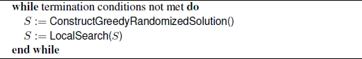
The greedy randomized adaptive search procedure (GRASP) [RES 10a] is a conceptually simple, but often effective, metaheuristic. As indicated by the name, the core of GRASP is based on the probabilistic construction of solutions. However, while ACO algorithms, for example, include a memory of the search history in terms of the pheromone model, GRASP does not make use of memory. More specifically, GRASP – as pseudo-coded in Algorithm 1.5 – combines the randomized greedy construction of solutions with the subsequent application of a local search. For the following discussion let us assume that, given a partial solution Sp, set Ext(Sp) ⊆ C is the set of solution components that may be used to extend Sp. The probabilistic construction of a solution using GRASP makes use of a so-called restricted candidate list L, which is a subset of Ext(Sp), at each step. In fact, L is determined to contain the best solution components from Ext(Sp) with respect to a greedy function. After generating L, a solution component c∗ ∈ L is chosen uniformly at random. An important parameter of GRASP is α, which is the length of the restricted candidate list L. If α = 1, for example, the solution construction is deterministic and the resulting solution is equal to the greedy solution. In the other extreme case – that is, when choosing α = |Ext(Sp)| – a random solution is generated without any heuristic bias. In summary, α is a critical parameter of GRASP which generally requires a careful fine-tuning.
Algorithm 1.5. Greedy randomized adaptive search procedure (GRASP)
As mentioned above, the second component of the algorithm consists of the application of local search to the solutions constructed. Note that, for this purpose, the use of a standard local search method such as the one from Algorithm 1.2 is the simplest option. More sophisticated options include, for example, the use of metaheuristics based on a local search such as simulated annealing. As a rule of thumb, the algorithm designer should take care that: (1) the solution construction mechanism samples promising regions of the search space: and (2) the solutions constructed are good starting points for a local search, i.e. the solutions constructed fall into basins of attraction for high-quality local minima.
1.2.4. Iterated local search
Iterated local search (ILS) [LOU 10] is – among the metaheuristics described in this section – the first local search extension. The idea of ILS is simple: instead of repeatedly applying local search to solutions generated independently from each other, as in GRASP, ILS produces the starting solutions for a local search by randomly perturbing the incumbent solutions. The requirements for the perturbation mechanism are as follows. The perturbed solutions should lie in a different basin of attraction with respect to the local search method utilized. However, at the same time, the perturbed solution should be closer to the previous incumbent solution than a randomly generated solution.
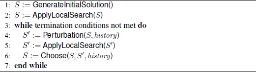
More specifically, the pseudo-code of ILS – as shown in Algorithm 1.6 – works as follows. First, an initial solution is produced in some way in the GenerateInitialSolution() function. This solution serves as input for the first application of a local search (see ApplyLocalSearch(S) function in line 2 of the pseudo-code). At each iteration, first, the perturbation mechanism is applied to the incumbent solution S; see Perturbation(S,history) function. The parameter history refers to the possible influence of the search history on this process. The perturbation mechanism is usually non-deterministic in order to avoid cycling, which refers to a situation in which the algorithm repeatedly returns to solutions already visited. Moreover, it is important to choose the perturbation strength carefully. This is, because: (1) a perturbation that causes very few changes might not enable the algorithm to escape from the current basin of attraction; (2) a perturbation that is too strong would make the algorithm similar to a random-restart local search. The last algorithmic component of ILS concerns the choice of the incumbent solution for the next iteration; see function Choose(S, S′, history). In most cases, ILS algorithms simply choose the better solution from among S and S′. However, other criteria – for example, ones that depend on the search history – might be applied.
Algorithm 1.6. Iterated local search (ILS)
1.2.5. Simulated annealing
Simulated annealing (SA) [NIK 10] is another metaheuristic that is an extension of local search. SA has – just like ILS – a strategy for escaping from the local optimal of the search space. The fundamental idea is to allow moves to solutions that are worse than the incumbent solution. Such a move is generally known as an uphill move. SA is inspired by the annealing process of metal and glass. When cooling down such materials from the fluid state to a solid state, the material loses energy and finally assumes a crystal structure. The perfection – or optimality – of this crystal structure depends on the speed at which the material is cooled down. The more carefully the material is cooled down, the more perfect the crystal structure. The first times that SA was presented as a search algorithm for CO problems was in [KIR 83] and in [CER 85].
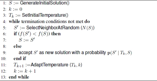
SA works as shown in Algorithm 1.7. At each iteration, a solution S′ ∈ N(S) is randomly selected. If S′ is better than S, then S′ replaces S as incumbent solution. Otherwise, if S is worse than S′ – that is, if the move from S to S′ is an uphill move – S′ may still be accepted as new incumbent solution with a positive probability that is a function of a temperature parameter Tk – in analogy to the natural inspiration of SA – and the difference between the objective function value of S′ and that of S (f(s′) − f(s)). Usually this probability is computed in accordance with Boltzmann’s distribution. Note that when SA is running, the value of Tk gradually decreases. In this way, the probability of accepting an uphill move decreases during run time.
Algorithm 1.7. Simulated annealing (SA)
Note that the SA search process can be modeled as a Markov chain [FEL 68]. This is because the trajectory of solutions visited by SA is such that the next solution is chosen depending only on the incumbent solution. This means that – just like GRASP – basic SA is a memory-less process.
1.2.6. Other metaheuristics
Apart from the five metaheuristics outlined in the previous sections, the literature offers a wide range of additional algorithms that fall under the metaheuristic paradigm. Examples are established metaheuristics, such as Tabu search [GLO 97, GEN 10b], particle swarm optimization [KEN 95, JOR 15], iterated greedy algorithms [HOO 15] and variable neighborhood search (VNS) [HAN 10]. More recent metaheuristics include artificial bee colony optimization [KAR 07, KAR 08] and chemical reaction optimization [LAM 12].
1.2.7. Hybrid approaches
Quite a large number of algorithms have been reported in recent years that do not follow the paradigm of a single traditional metaheuristic. They combine various algorithmic components, often taken from algorithms from various different areas of optimization. These approaches are commonly referred to as hybrid metaheuristics. The main motivation behind the hybridization of different algorithms is to exploit the complementary character of different optimization strategies, i.e. hybrids are believed to benefit from synergy. In fact, choosing an adequate combination of complementary algorithmic concepts can be the key to achieving top performance when solving many hard optimization problems. This has also seen to be the case in the context of string problems in bioinformatics, for example in the context of longest common subsequence problems in Chapter 3. In the following section, we will mention the main ideas behind two generally applicable hybrid metaheuristics from the literature: large neighborhood search (LNS), and construct, merge, solve & adapt (CMSA). A comprehensive introduction into the field of hybrid metaheuristics is provided, for example, in [BLU 16e].
1.2.7.1. Large neighborhood search
The LNS Algorithm (see [PIS 10] for an introduction) was introduced based on the following observation. As complete solvers are often only efficient for small to medium size problems, the following general idea might work very well. Given a problem for which the complete solver under consideration is no efficient longer, we generate a feasible solution in some way – for example, by means of a constructive heuristic – and try to improve this solution in the following way. First, we partially destroy the solution by removing some components of the solution. This can either be done in a purely random way or guided by a heuristic criterion. Afterwards, the complete solver is applied to the problem of finding the best valid solution to the original problem that includes all solution components of the given partial solution. As a partial solution is already given, the complexity of this problem is significantly lower and the complete solver might be efficiently used to solve it. This procedure is iteratively applied to an incumbent solution. In this way, LNS still profits from the advantages of the complete solver, even in the context of large problems.
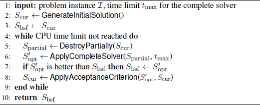
The pseudo-code of a general LNS algorithm is provided in Algorithm 1.8. First, in line 2 of Algorithm 1.8, an initial incumbent solution Scur is generated in the GenerateInitialSolution() function. This solution (Scur) is then partially destroyed at each iteration, for example by removing some of its components. The number (or percentage) of components to be removed, as well as how these components are chosen, are important design decisions. The resulting partial solution Spartial is fed to a complete solver; see function ApplyCompleteSolver(Spartial, tmax) in line 6 of Algorithm 1.8. This function includes the current partial solution Spartial and a time limit tmax. Note that the complete solver is forced to include Spartial in any solution considered. The complete solver provides the best valid solution found within the computation time available tmax. This solution, denoted by ![]() , may or may not be the optimal solution to the subproblem tackled. This depends on the given computation time limit tmax for each application of the complete solver. Finally, the last step of each iteration consists of a choice between Scur and
, may or may not be the optimal solution to the subproblem tackled. This depends on the given computation time limit tmax for each application of the complete solver. Finally, the last step of each iteration consists of a choice between Scur and ![]() to be the incumbent solution of the next iteration. Possible options are: (1) selecting the better one among the two; or (2) applying a probabilistic choice criterion.
to be the incumbent solution of the next iteration. Possible options are: (1) selecting the better one among the two; or (2) applying a probabilistic choice criterion.
1.2.7.2. Construct, merge, solve and adapt
The CMSA algorithm was introduced in [BLU 16b] with the same motivation that had already led to the development of LNS as outlined in the previous section. More specifically, the CMSA algorithm is designed in order to be able to profit from an efficient complete solver even in the context of problem that are too large to be directly solved by the complete solver. The general idea of CMSA is as follows. At each iteration, solutions to the problem tackled are generated in a probabilistic way. The components found in these solutions are then added to a sub-instance of the original problem. Subsequently, an exact solver such as, for example, CPLEX is used to solve the sub-instance to an optimal level. Moreover, the algorithm is equipped with a mechanism for deleting seemingly useless solution components from the sub-instance. This is done such that the sub-instance has a moderate size and can be quickly and optimally solved.
Algorithm 1.8. Large neighborhood search (LNS)
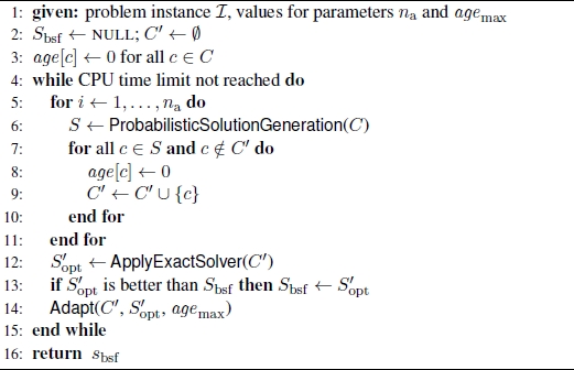
The pseudo-code of the CMSA algorithm is provided in Algorithm 1.9. Each algorithm iteration consists of the following actions. First, the best-so-far solution Sbsf is set to NULL, indicating that no such solution yet exists. Moreover, the restricted problem, C′, which is simply a subset of the complete set, C, of solution components is set to the empty set2. Then, at each iteration, na solutions are probabilistically generated in function ProbabilisticSolutionGeneration(C); see line 6 of Algorithm 1.9. The components found in the solutions constructed are then added to C′. The so-called age of each of these solution components (age[c]) is set to 0. Next, a complete solver is applied in function ApplyExactSolver(C′) to find a possible optimal solution ![]() to the restricted problem C′. If
to the restricted problem C′. If ![]() is better than the current best-so-far solution Sbsf, solution
is better than the current best-so-far solution Sbsf, solution ![]() is taken as the new best-so-far solution. Next, sub-instance C′ is adapted on the basis of solution
is taken as the new best-so-far solution. Next, sub-instance C′ is adapted on the basis of solution ![]() in conjunction with the age values of the solution components; see function Adapt(C′,
in conjunction with the age values of the solution components; see function Adapt(C′, ![]() , agemax) in line 14. This is done as follows. First, the age of each solution component in C′
, agemax) in line 14. This is done as follows. First, the age of each solution component in C′ ![]() is incremented while the age of each solution component in
is incremented while the age of each solution component in ![]() ⊆ C′ is re-set to zero. Subsequently, those solution components from C′ with an age value greater than agemax – which is a parameter of the algorithm – are removed from C′. This means that solution components that never appear in solutions derived by the complete solver do not slow down the solver in subsequent iterations. Components which appear in the solutions returned by the complete solver should be maintained in C′.
⊆ C′ is re-set to zero. Subsequently, those solution components from C′ with an age value greater than agemax – which is a parameter of the algorithm – are removed from C′. This means that solution components that never appear in solutions derived by the complete solver do not slow down the solver in subsequent iterations. Components which appear in the solutions returned by the complete solver should be maintained in C′.
Algorithm 1.9. Construct, merge, solve & adapt (CMSA)
1.3. Outline of the book
The techniques outlined in the previous sections have been used extensively over recent decades to solve CO problems based on strings in the field of bioinformatics. Examples of such optimization problems dealing with strings include the longest common subsequence problem and its variants [HSU 84, SMI 81], string selection problems [MEN 05, MOU 12a, PAP 13], alignment problems [GUS 97, RAJ 01a] and similarity search [RAJ 01b]. We will focus on a collection of selected string problems and recent techniques for solving them in this book:
- – Chapter 2 is concerned with a CO problem known as the unbalanced minimum common string partition (UMCSP) problem. This problem is a generalization of the minimum common string partition (MCSP) problem. First, an ILP model for the UMCSP problem is presented. Second, a simple greedy heuristic initially introduced for the MCSP problem is adapted to be applied to the UMCSP problem. Third, the application of the hybrid metaheuristic, CMSA (see section 1.2.7.2 for a general description of this technique), to the UMCSP problem is described. The results clearly show that the CMSA algorithm outperforms the greedy approach. Moreover, they show that the CMSA algorithm is competitive with CPLEX for small and medium problems whereas it outperforms CPLEX for larger problems.
- – Chapter 3 deals with a family of string problems that are quite common in bio-informatics applications: longest common subsequence (LCS) problems. The most general problem from this class is simply known as the LCS problem. Apart from the general LCS problem, there is a whole range of specific problems that are mostly restricted cases of the general LCS problem. In this chapter we present the best available algorithms for solving the general LCS problem. In addition, we will deal with a specific restriction known as the repetition-free longest common subsequence (RFLCS) problem. An important landmark in the development of metaheuristics for LCS problems was the application of beam search to the general LCS problem in 2009 [BLU 09]. This algorithm significantly outperformed any other algorithm that was known at this time. Moreover, most algorithms proposed afterwards are based on this original beam search approach. After a description of the original beam search algorithm, Chapter 3 presents a hybrid metaheuristic called Beam–ACO. This algorithm is obtained by combining the ACO metaheuristic with beam search. Subsequently, the current state-of-the-art metaheuristic for the RFLCS problem is described. This algorithm is also a hybrid metaheuristic obtained by combining probabilistic solution construction with the application of an ILP solver to solve sub-instances of the original problem (see section 1.2.7.2 for a general description of this technique).
- – Chapter 4 deals with an NP-hard string selection problem known as the most strings with few bad columns (MSFBC) problem. This problem models the following situation: a set of DNA sequences from a heterogeneous population consisting of two subgroups: (1) a large subset of DNA sequences that are identical apart from at most k positions at which mutations may have occurred; and (2) a subset of outliers. The goal of the MSFBC problem is to separate the two subsets. First, an ILP model for the MSFBC problem is described. Second, two variants of a rather simple greedy strategy are outlined. Finally, the current state-of-the-art metaheuristic for the MSFBC problem, which is a LNS approach, is described. The LNS algorithm makes use of the ILP solver CPLEX as a sub-routine in order to find, at each iteration, the best neighbor in a large neighborhood of the current solution. A comprehensive experimental comparison of these techniques shows that LNS, generally, outperforms both greedy strategies. While LNS is competitive with the stand-alone application of CPLEX for small and medium size problems, it outperforms CPLEX in the context of larger problems.
- – Chapter 5 provides an overview over the best metaheuristic approaches for solving string selection and comparison problems, with a special emphasis on so-called consensus string problems. The intrinsic properties of the problems are outlined and the most popular solution techniques overviewed, including some recently-proposed heuristic and metaheuristic approaches. It also proposes a simple and efficient ILP-based heuristic that can be used for any of the problems considered. Future directions are discussed in the last section.
- – Chapter 6 deals with the pairwise and the multiple alignment problems. Solution techniques are discussed, with special emphasis on the CO perspective, with the goal of providing conceptual insights and referencing literature produced by the broad community of researchers and practitioners.
- – Finally, the last chapter describes the best metaheuristic approaches for some other string problems that are not dealt with in this book in more detail, such as several variants of DNA sequencing and the founder sequence reconstruction problem.