
4
The Most Strings With Few Bad Columns Problem
This chapter deals with an non-deterministic polynomial-time (NP)-hard string selection problem known as the most strings with few bad columns (MSFBC) problem. The problem was originally introduced as a model for a set of DNA sequences from a heterogeneous population consisting of two subgroups: (1) a rather large subset of DNA sequences that are identical apart from mutations at maximal k positions; and (2) a smaller subset of DNA sequences that are outliers. The goal of the MSFBC problem is to identify the outliers. In this chapter, the first and foremost problem is modeled by means of integer linear programming (ILP). Second, two variants of a rather simple greedy strategy are outlined. Finally, a large neighborhood search (LNS) approach (see section 1.2.7.1 for a general introduction to LNS) for the MSFBC problem is described. This approach is currently the state-of-the-art technique. The LNS algorithm makes use of the ILP solver CPLEX as a sub-routine in order to find, at each iteration, the best possible neighbor in a large neighborhood of the current solution. A comprehensive experimental comparison among these techniques shows, first, that LNS generally outperforms both greedy strategies. Second, while LNS is competitive with the stand-alone application of CPLEX for small and medium size problems, it outperforms CPLEX in the context of larger problems. Note that the content of this chapter is based on [LIZ 16].
As already described in section 1.2.7.1, LNS algorithms are based on the following general idea. Given a valid solution to the problem tackled – also called the incumbent solution – first, destroy selected parts of it, resulting in a partial solution. Then apply some other, possibly exact, technique to find the best valid solution on the basis of the partial solution, i.e. the best valid solution that contains the given partial solution. Thus, the destroy-step defines a large neighborhood, from which the best (or nearly best) solution is determined not by naive enumeration but by the application of a more effective alternative technique. In the case of the MSFBC problem, the LNS algorithm makes use of the ILP-solver CPLEX to explore large neighborhoods. Therefore, the LNS approach can be labeled an ILP-based LNS.
4.1. The MSFBC problem
The MSFBC problem was originally introduced in [BOU 13]. It can, technically, be described as follows. A set I of n input strings of length m over a finite alphabet Σ, i.e. I = {s1, … , sn}. The j-th position of a string si is, henceforth, denoted by si[j] and has a k < m fixed value. Set I together with parameter k define problem (I, k). The goal is to find a subset S ⊆ I of maximal size such that the strings in S differ in at most k positions. In this context, the strings of a subset S ⊆ I are said to differ in position 1 ≤ j ≤ m if, and only if, at least two strings si, sr ∈ s exist where ![]() . A position j in which the strings from S differ is also called a bad column. This notation is derived from the fact that the set of input strings can conveniently be seen in the form of a matrix in which the strings are the rows.
. A position j in which the strings from S differ is also called a bad column. This notation is derived from the fact that the set of input strings can conveniently be seen in the form of a matrix in which the strings are the rows.
4.1.1. Literature review
The authors of [BOU 13] showed that no polynomial-time approximation scheme (PTAS) exists for the MSFBC problem. Moreover, they state that the problem is a generalization of the problem of finding tandem repeats in a string [LAN 01]. In [LIZ 15], the authors introduced the first ILP model for the MSFBC problem (see section 4.2). They devised a greedy strategy which was tested in the context of a pilot method [VOß 05]. For problems of small and medium size, the best results were obtained by solving the ILP model by CPLEX, while the greedy-based pilot method scaled much better to large problems. On the downside, the greedy-based pilot method consumed a rather large amount of computation time.
4.2. An ILP model for the MSFBC problem
To describe the ILP model, let Σj ⊆ Σ be the set of letters appearing at least once at the j-th position of the n input strings. In technical terms, Σj := {si[j] | i = 1, … , n}. The proposed ILP model for the MSFBC problem makes use of several types of binary variable. First, for each input string si there is a binary variable xi. Where xi = 1, the corresponding input string si is part of the solution, otherwise not. Furthermore, for each combination of position j (j = 1, … , m) and letter a ∈ Σj the model makes use of a binary variable ![]() , which is forced – by means of adequate constraints – to assume a value of one
, which is forced – by means of adequate constraints – to assume a value of one ![]() where at least one string si with si[j] = a is chosen for the solution. Finally, there is a binary variable yj for each position j = 1, … , m. Variable yj is forced to assume a value of one (yj = 1) where the strings chosen for the solution differ at position j. Given these variables, the ILP can be formulated as follows:
where at least one string si with si[j] = a is chosen for the solution. Finally, there is a binary variable yj for each position j = 1, … , m. Variable yj is forced to assume a value of one (yj = 1) where the strings chosen for the solution differ at position j. Given these variables, the ILP can be formulated as follows:
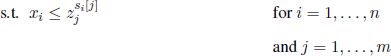
The objective function [4.1] maximizes the number of strings chosen. Equations [4.2] ensure that, if a string si is selected (xi = 1), the variable ![]() , which indicates that letter si[j] appears at position j in at least one of the selected strings, has a value of one. Furthermore, equations [4.3] ensure that yj is set to one when the selected strings differ at position j. Finally, constraint [4.4] ensures that no more than k bad columns are permitted.
, which indicates that letter si[j] appears at position j in at least one of the selected strings, has a value of one. Furthermore, equations [4.3] ensure that yj is set to one when the selected strings differ at position j. Finally, constraint [4.4] ensures that no more than k bad columns are permitted.
4.3. Heuristic approaches
Given a non-empty partial solution to the problem, the authors of [LIZ 15] proposed the following greedy strategy to complete the partial solution given. In this context, bc(Sp) denotes the number of bad columns with respect to a given partial solution Sp ⊆ I. This measure corresponds to the number of columns j such that at least two strings si, sr ∈ Sp exist where si[j] =sr[j]. A valid partial solution Sp to the MSWBC problem fulfills the following two conditions:
1) bc(Sp) ≤ k;
2) There is at least one string sl ∈ I Sp where bc(Sp ∪ {sl}) ≤ k.
It is not difficult to see that a valid complete solution S fulfills only the first of these conditions.
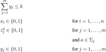
Algorithm 4.1. MakeSolutionComplete(Sp) procedure
The pseudo-code of the MakeSolutionComplete(Sp) procedure for completing a given partial solution is provided in Algorithm 4.1. It works in an iterative way, whereby in each iteration exactly one of the strings from I Sp is chosen. This is done by making use of a weighting function. The chosen string is then added to Sp. The weighting function concerns the number of bad columns. From E := {s ∈ I Sp | bc(Sp ∪ {s}) ≤ k} strings, the one with minimum bc(Sp ∪ {s}) is selected. In other words, at each iteration the string that causes a minimum increase in the number of bad columns is selected. In case of ties, the first one encountered is selected.
4.3.1. Frequency-based greedy
The authors of [LIZ 15] proposed two different ways of using the MakeSolutionComplete(Sp) procedure. In the first one, the initial partial solution contains exactly one string that is chosen based on a criterion related to letter frequencies. Let frj,a for all a ∈ Σ and j = 1, … , m be the frequency of letter a at position j in the input strings from I. If a appears, for example, in five out of n input strings at position j, then frj,a = 5/n. With this definition, the following measure can be computed for each si ∈ I:
where si[j] denotes the letter at position j of string si. In words, ω(si) is calculated as the sum of the frequencies of the letters in si. The following string is, then, chosen to form the partial solution used as input for the MakeSolutionComplete(Sp) procedure:
The advantages of this greedy algorithm – denoted by GREEDY-F – are to be found in its simplicity and low resource requirements.
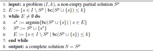
4.3.2. Truncated pilot method
The MakeSolutionComplete(Sp) procedure was also used in [LIZ 15] in the context of a pilot method in which the MakeSolutionComplete(Sp) procedure was used at each level of the search tree in order to evaluate the respective partial solutions. The choice of a partial solution at each level was made on the basis of these evaluations. The computation time of such a pilot method is exponential in comparison to the basic greedy method. One way of reducing the computation time is to truncate the pilot method. Among several truncation options, the one with the best balance between solution quality and computation time in the context of the MSFBC problem is shown in Algorithm 4.2. For each possible string of si ∈ I, the resulting partial solution Sp = {si} is fed in to the MakeSolutionComplete(Sp) procedure. The output of the truncated pilot method, henceforth called PILOT-TR, is the best of the n solutions constructed in this way.
Algorithm 4.2. Truncated pilot method
4.4. ILP-based large neighborhood search
In [LIZ 15], CPLEX was applied to a range of MSFBC problems. In this context, it was observed that CPLEX failed to provide near-optimal solutions for large problems. ILP-based LNS is a popular technique for profiting from CPLEX even with large problems are concerned. In the following, such an ILP-based LNS algorithm is described for application to the MSFBC problem. At each iteration, the current solution is initially partially destroyed. This may be done in a purely random way, or with some heuristic bias. The result, in any case, is a partial solution to the problem tackled. Then, CPLEX is applied to find the best valid solution that contains the partial solution obtained in the destruction step. Given a partial solution Sp, the best complete solution containing Sp is obtained by applying CPLEX to the ILP model from section 4.2, augmented by the following set of constraints:
The pseudo-code of the ILP-based LNS algorithm is shown in Algorithm 4.3. First, in line 2, the first incumbent solution Sbsf is generated by applying heuristic GREEDY-F from section 4.3.1 to the problem tackled (I, k). Second, the current incumbent solution Sbsf is partially destroyed (see line 5) by removing a certain percentage percdest of the strings in Sbsf. This results in a partial solution Sp. After initial experiments it was decided to choose the strings to be removed uniformly at random. The precise number d of strings to be removed is calculated on the basis of percdest as follows:
The last step of each iteration consists of applying the ILP solver CPLEX to produce the best solution, ![]() , containing the partial solution Sp (see line 6). To avoid that this step taking too much computation time, CPLEX is given a computation time limit of tmax seconds. The output of CPLEX is, therefore, the best – possibly optimal – solution found within the computation time allowed.
, containing the partial solution Sp (see line 6). To avoid that this step taking too much computation time, CPLEX is given a computation time limit of tmax seconds. The output of CPLEX is, therefore, the best – possibly optimal – solution found within the computation time allowed.
Algorithm 4.3. ILP-based LNS for the MSFBC problem
To provide the algorithm with a way to escape from local optima, the percentage percdest of strings to be removed from the current solution is variable and depends on the search history. Two additional parameters are introduced for this purpose: a lower bound ![]() and an upper bound
and an upper bound ![]() . For the values of these bounds it holds that
. For the values of these bounds it holds that ![]() .
.
Initially, the value of percdest is set to the lower bound (see line 3 of Algorithm 4.3). Then, at each iteration, if the solution ![]() produced by CPLEX is better than Sbsf, the value of percdest is set to the lower bound
produced by CPLEX is better than Sbsf, the value of percdest is set to the lower bound ![]() . If this is not the case, the value of percdest is incremented by a certain amount. For the experimental evaluation presented in this chapter, this
. If this is not the case, the value of percdest is incremented by a certain amount. For the experimental evaluation presented in this chapter, this ![]() constant was set to five. If the value of percdest exceeds the upper bound , it is set to the lower bound
constant was set to five. If the value of percdest exceeds the upper bound , it is set to the lower bound ![]() . This mechanism is described in lines 7–15 of the pseudo-code.
. This mechanism is described in lines 7–15 of the pseudo-code.
Note that the idea behind the dynamic change of the value of percdest is as follows. As long as the algorithm is capable of improving the current solution bsf using a low destruction percentage, this percentage is kept low. In this way, the large neighborhood is rather small and CPLEX is faster in deriving the corresponding optimal solutions. Only when the algorithm does not seem to be able to improve over the current solution Sbsf is the destruction percentage is increased in a step-wise way.
4.5. Experimental evaluation
This section presents a comprehensive experimental evaluation of four algorithmic approaches: (1) the frequency-based greedy method GREEDY-F from section 4.3.1; (2) the truncated pilot method PILOT-TR from section 4.3.2; (3) the large neighborhood search (LNS) approach from section 4.4; and (4) the application of CPLEX to all problems. All approaches were implemented in ANSI C++ using GCC 4.7.3 to compile the software. Moreover, the original ILPs as well as the ILPs within LNS were solved with IBM ILOG CPLEX V12.2 (single-threaded execution). The experimental results that are presented were obtained on a cluster of computers with Intel® Xeon® CPU 5670 CPUs of 12 nuclei of 2933 MHz and (in total) 32 GB of RAM. A maximum of 4 GB of RAM was allowed for each run of CPLEX. In the following section, the set of benchmarks is described. A detailed analysis of the experimental results is presented thereafter.
4.5.1. Benchmarks
For the experimental comparison of the methods considered in this chapter, a set of random problems was generated on the basis of four different parameters: (1) the number of input strings (n); (2) the length of the input strings (m); (3) the alphabet size (|Σ|); and (4) the so-called change probability (pc). Each random instance is generated as follows. First, a base string s of length m is generated uniformly at random, i.e. each letter a ∈ Σ has a probability of 1/|Σ| to appear at any of the m positions of s. Then, the following procedure is repeated n times in order to generate n input strings of the problem being constructed. First, s is copied into a new string s'. Then, each letter of s' is exchanged with a randomly chosen letter from Σ with a probability of pc. Note that the new letter does not need to be different from the original one. However, note that at least one change per input string was enforced.
The following values were used for the generation of the benchmark set:
- − n ∈ { 100, 500, 1000 };
- − m∈ { 100, 500, 1000 };
- − |Σ| ∈ { 4, 12, 20 }.
Values for pc were chosen in relation to n:
- 1) If n = 100: pc ∈ {0.01, 0.03, 0.05};
- 2) If n = 500: pc ∈ {0.005, 0.015, 0.025};
- 3) If n = 1000: pc ∈ {0.001, 0.003, 0.005}.
The three chosen values for pc imply for any string length that, on average, 1%, 3% or 5% of the string positions are changed. Ten problems were generated for each combination of values for parameters n, m and |Σ|. This results in a total of 810 benchmarks. To test each instance with different limits for the number of bad columns allowed, values for k from {2, n/20, n/10} were used.
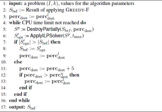
Table 4.1. Parameter settings produced by irace for LNS concerning |Σ| = 4
4.5.2. Tuning of LNS
The LNS parameters were tuned by means of the automatic configuration tool irace [LÓP 11]. The parameters subject to tuning were: (1) the lower and upper bounds – that is, ![]() and
and ![]() – of the percentage of strings to be deleted from the current incumbent solution Sbsf; and (2) the maximum time tmax (in seconds) allowed for CPLEX per application within LNS. irace was applied separately for each combination of values for n, |Σ| and k, respectively. Note that no separate tuning was performed concerning the string length m and the percentage of character change pc. This is because, after initial runs, it was shown that parameters n, |Σ| and k have as large an influence on the behavior of the algorithm as m and pc. irace was applied 27 times with a budget of 1,000 applications of LNS per tuning run. For each application of LNS, a time limit of n/2 CPU seconds was given. Finally, for each of irace run, one tuning instance for each combination of m and pc was generated. This makes a total of 9 tuning instances per of irace run.
– of the percentage of strings to be deleted from the current incumbent solution Sbsf; and (2) the maximum time tmax (in seconds) allowed for CPLEX per application within LNS. irace was applied separately for each combination of values for n, |Σ| and k, respectively. Note that no separate tuning was performed concerning the string length m and the percentage of character change pc. This is because, after initial runs, it was shown that parameters n, |Σ| and k have as large an influence on the behavior of the algorithm as m and pc. irace was applied 27 times with a budget of 1,000 applications of LNS per tuning run. For each application of LNS, a time limit of n/2 CPU seconds was given. Finally, for each of irace run, one tuning instance for each combination of m and pc was generated. This makes a total of 9 tuning instances per of irace run.
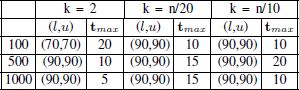
Table 4.2. Parameter settings produced by irace for LNS where |Σ| = 12
Finally, the parameter value ranges that were chosen for the LNS tuning processes are as follows:
– for the lower and upper bound values of the percentage destroyed, the following value combinations were considered: ![]() ∈ {(10,10), (20,20), (30,30), (40,40), (50,50), (60,60), (70,70), (80,80), (90,90), (10,30), (10,50), (30,50), (30,70)}. Note that in the cases where both bounds have the same value, the percentage of deleted nodes is always the same;
∈ {(10,10), (20,20), (30,30), (40,40), (50,50), (60,60), (70,70), (80,80), (90,90), (10,30), (10,50), (30,50), (30,70)}. Note that in the cases where both bounds have the same value, the percentage of deleted nodes is always the same;
– tmax ∈ {5.0, 10.0, 15.0, 20.0}.
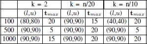
The results of the tuning processes are shown in Tables 4.1, 4.2 and 4.3. The following observations can be made. First, in nearly all cases (90, 90) is chosen for the lower and upper bounds of the percentage destroyed. This is surprising, because LNS algorithms generally require a lower of percentage destruction. At the end of section 4.5.3, some reasons will be outlined to explain this high percentage destruction in the MSFBC problem. No clear trend can be extracted from the settings chosen for tmax. The reason for this is related to the reason for choosing a high percentage destruction, which will be outlined later, as mentioned above.
Table 4.3. Parameter settings produced by irace for LNS where |Σ| = 20
4.5.3. Results
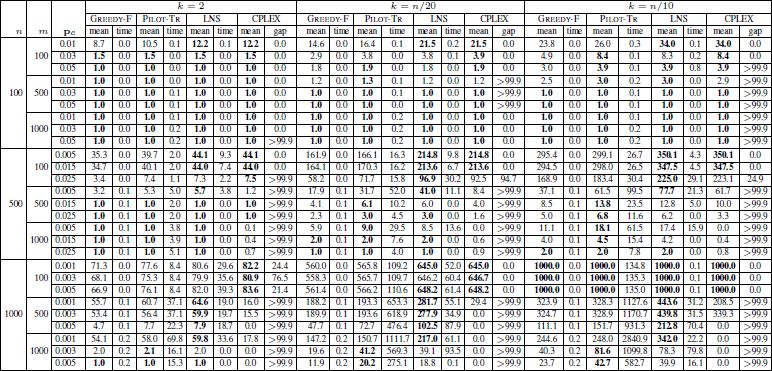
The results are provided numerically in three tables: Table 4.4 provides the results for all instances with |Σ| = 4; Table 4.5 contains the results for all instances with |Σ| = 12; and Table 4.6 shows the results for instances with |Σ| = 20. The first three columns contain the number of input strings (n), string length (m) and the probability of change (pc). The results of GREEDY-F, PILOT-TR, LNS and CPLEX are presented in the three blocks of columns, each one corresponding to one of the three values for k. In each of these blocks, the tables provide the average results obtained for 10 random instances in each row (columns with the heading “mean”) and the corresponding average computation times in seconds (columns with the heading “time”). Note that LNS was applied with a time limit of n/2 CPU seconds for each problem. With CPLEX, which was applied with the same time limits as LNS, the average result (column with the heading “mean”) and the corresponding average optimality gap (column with the heading “gap”) is provided. Note that when the gap has a value of zero, the 10 corresponding problems were optimally solved within the computation time allowed. Finally, note that the best result in each row is marked in bold font.
Table 4.4. Experimental results for instances where |Σ| = 4
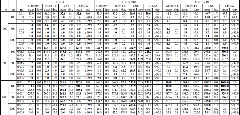
Table 4.5. Experimental results for instances where |Σ| = 12
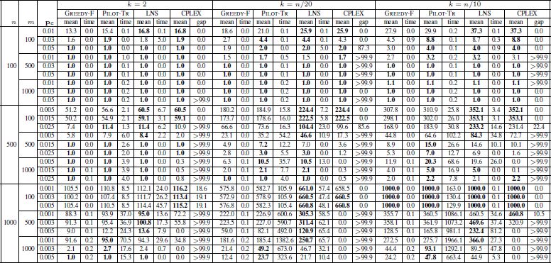
Table 4.6. Experimental results for instances where |Σ| = 20
In addition to the numerical results, Figure 4.1 shows the improvement of LNS over PILOT-TR and Figure 4.2 shows the improvement of LNS over CPLEX. X, Y and Z take values from {S, M, L}, where S refers to small, M refers to medium and L refers to large. While X refers to the number of input strings, Y refers to their length and Z to the probability of change. In positions X and Y , S refers to 100, M to 500 and L to 1000, while in the case of Z, S refers to {0.01, 0.005, 0.001}, M to {0.03, 0.015, 0.003} and L to {0.05, 0.025, 0.005}, depending on the value of n.
The following observations can be made on the basis of the results:
- – alphabet size does not seem to play a role in the relative performance of the algorithms. An increasing alphabet size decreases the objective function values;
- – PILOT-TR and LNS outperform GREEDY-F. It is beneficial to start the greedy strategy from n different partial solutions (each one containing exactly one of the n input strings) instead of applying the greedy strategy to the partial solution containing the string obtained by the frequency-based mechanism;
- – LNS and PILOT-TR perform comparably for small problems. When large problems are concerned, especially in the case of |Σ| = 4, LNS generally outperforms PILOT-TR. However, there are some noticeable exceptions, especially for L-S-S and L-L-S in Figure 4.1(b) and L-L-S in Figure 4.1(c), i.e. when k = 2 and problems are large, PILOT-TR sometimes performs better than LNS;
- – with LNS the relative behavior that is to be expected and CPLEX is displayed in Figure 4.2. LNS is competitive with CPLEX for small and medium instances all alphabet sizes and for all values of k. Moreover, LNS generally outperforms CPLEX in the context of larger problems. This is, again, with the exception of L-S-∗ in the case of |Σ| ∈ {12, 20} for k = 2, where CPLEX performs slightly better than LNS;
- – CPLEX requires substantially more computation time than LNS, GREEDY-R and PILOT-TR to reach solutions of similar quality.
In summary, LNS is currently the state-of-the-art method for the MSFBC problem. The disadvantages of LNS in comparison to PILOT-TR and CPLEX, for instance, where |Σ| ∈ {12, 20} and k = 2, leave room for further improvement.
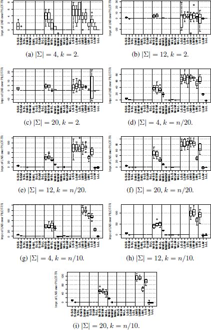
Figure 4.1. Improvement of LNS over PILOT-TR (in absolute terms). Each box shows these differences for the corresponding 10 instances. Note that negative values indicate that PILOT-TR obtained a better result than LNS
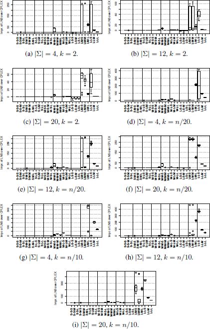
Figure 4.2. Improvement of LNS over CPLEX (in absolute terms). Each box shows these differences for the corresponding 10 instances. Note that negative values indicate that CPLEX obtained a better result than LNS
Finally, it is interesting to study the reasons that the tuning procedure (irace) has a very high percentage of destruction in nearly all cases. Remember that this is rather unusual for a LNS algorithm. To shed some light on this matter, LNS was applied for 100 iterations in two exemplary cases: (1) a problem with n = 500, m = 100, pc = 0.015, |Σ| = 4; and k = n/20; and (2) a problem with n = 1000, m = 500, pc = 0.003, |Σ| = 4 and k = n/20. This was done in both cases for fixed destruction over the whole range between 10% and 90%. In all runs, the average times needed by CPLEX to obtain optimal solutions when applied to the partial solution of each iteration was measured. The average times (together with the corresponding standard deviations) are displayed in Figure 4.3. It can be observed, in both cases, that CPLEX is very fast for any percentage destruction. In fact, the time difference betweens 10% and 90% destruction is nearly negligible. Moreover, note that CPLEX requires 18.1 seconds to solve the original problem optimally, whereas in the second case CPLEX is not able to find a solution with an optimality gap below 100 within 250 CPU seconds. This implies that in the case of the MSFBC problem, as long as a small partial solution is given, CPLEX is very fast in deriving the optimal solution that contains the respective partial solution. Moreover, there is hardly any difference in the computation time requirements with respect to the size of this partial solution. This is the main reason why irace chose a large destruction percentage in nearly all cases. This also implies that the computation time limit given to CPLEX within LNS hardly plays any role. In other words, all computation time limits considered were sufficient for CPLEX when applied within LNS. This is why no tendency can be observed in the values chosen by irace for tmax.
4.6. Future work
Future work in the context of the MSFBC problem should exploit the following property: even when fed with very small partial solutions, CPLEX is often very fast in deriving the best possible solution containing a partial solution. In fact, a simple heuristic that profits from this property would start, for example, with the first string chosen by the frequency-based greedy method and would feed the resulting partial solution to CPLEX.
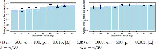
Figure 4.3. Average time (in seconds) used by CPLEX within LNS for each application at each iteration. Two examples considering destruction between 10 and 90 percent
Another line for future research includes the exploration of other, alternative, ways of combining metaheuristic strategies with CPLEX. One option concerns the use of CPLEX to derive a complete solution on the basis of a partial solution within the recombination operator of an evolutionary algorithm.