
6
Alignment Problems
This chapter provides an overview of pairwise and multiple alignment problems. Solution techniques are discussed, with special emphasis on combinatorial optimization (CO), with the goal of providing conceptual insights and references to literature written by a broad community of researchers and practitioners.
6.1. Introduction
Real-world systems and phenomena are often conveniently represented by strings and sequences of symbols, as is the case of spins in magnetic unidimensional systems, or sequences of bits in the recording and transmission of digital data. Analysis of a sequence of symbols aims to extrapolate from it the information that it carries, i.e. its properties and characteristics. In the field of molecular biology, DNA and RNA strings have an immediate and intrinsic interpretation as sequences of symbols and, for example, one may be interested in determining the activity of specific subsequences. Since researchers in molecular biology claim that similar primary biological structures correspond to similar activities, techniques that compare sequences are used to obtain information about an unknown sequence from the knowledge of two or more sequences that have already been. Comparing genomic sequences drawn from individuals from different species consists of determining their similarity or difference. Such comparisons are needed to identify not only functionally relevant DNA regions, but also spot fatal mutations and evolutionary relationships. To compute the similarity between protein and amino acid sequences is, in general, a computationally intractable problem. Moreover, the concept of similarity itself does not have a single definition. Proteins and DNA segments can be considered similar in several different ways. They can have a similar structure or can have a similar primary amino acid sequence. Given two linearly-ordered sequences, one evaluates their similarity through a measure that associates a pair of sequences with a number related to the cardinality of subsets of corresponding elements/symbols (alignment). The correspondence must be order-preserving, i.e. if the i-th element of the first sequence s corresponds to the k-th element of the second sequence t, no element following i in s can correspond to an element preceding k in t. Furthermore, an element can be aligned with a blank or gap (‘-’) and two gaps cannot be aligned. Figure 6.1 shows a possible alignment of two sequences.
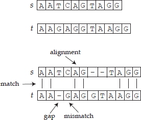
Figure 6.1. An example of alignment of two sequences
6.1.1. Organization of this chapter
The remainder of this chapter is organized as follows. Sections 6.2 and 6.3 are devoted to the pairwise and multiple alignment problem, respectively. These problems are mathematically formulated, their properties are described, and the most popular techniques to solve them are surveyed. Future directions are discussed in the last section.
6.2. The pairwise alignment problem
The simplest, computationally-tractable family of alignment problems concern the pairwise alignment of two sequences, s and t, considering only contiguous substrings with no internal deletions and/or insertions. The more general problem has been solved with methods developed to measure the minimum number of “events” needed to transform one string into another.
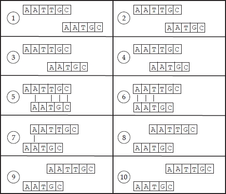
Figure 6.2. All possible alignments of two sequences without gaps
A naïve algorithm that computes all possible alignments of two sequences without the insertion of gaps simply slides one sequence along the other, and for each configuration it counts the number of letters that are exactly paired. Figure 6.2 shows the ten different possible alignments without gaps of two sequences with a length of 5 and 6 characters, respectively. With exactly four pairings, the alignment shown in number 5 is the best. Note that the concept of best alignment is clearly related to the criterion used to assess similarity. In general, the alignment with the largest number of matches (pairings) is considered to be best. The number of different alignments between two sequences of length n and m, is n + m − 1, under the assumption that no gaps can be inserted. Since for each possible alignment, each letter of the first sequence must be compared with each letter of the second sequence, the total computational complexity is O(n × m).
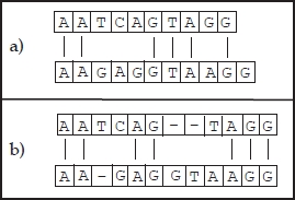
Figure 6.3. Two possible alignments of two sequences: a) not inserting gaps with 6 pairings; b) inserting gaps with 7 pairings
The possibility of inserting gaps strongly affects the quality of the solution obtained. See, for example, the two alignments depicted in Figure 6.3: alignment (a) does not allow the insertion of gaps and has 6 pairings while alignment (b) works with gaps and has 7 pairings. Nevertheless, the insertion of gaps influences the computational complexity of an algorithm that computes the best alignment. It is easy to understand that a naïve algorithm sliding one sequence along the other one is no longer suitable when considering gaps. This is because the number of different, gapped sequences that can be produced from an input sequence is exponential. Therefore, the design of more efficient alignment algorithms, such as the ones described in section 6.2.1, has been fundamental. Needleman and Wunsch’s algorithm is among the first methods that was proposed [NEE 70]. This algorithm uses a simple iterative matrix method of calculation. Later, Sankoff [SAN 72] and Reichert et al. [REI 73] proposed – from a mathematical point of view – more complex methods, but unfortunately they are not able to perfectly represent real biological scenarios. In 1974, Sellers [SEL 74] proposed a true metric measure of distance between strings, later generalized by Waterman et al. [WAT 76] to consider deletions/insertions of arbitrary length. In 1981, Smith and Waterman [SMI 81] extended the above ideas to design a dynamic programming algorithm able to determine the pair of segments of the two strings given with maximum similarity. This algorithm is outlined in section 6.2.1.
A simple graphical representation of the alignment of two sequences, called a dot matrix, was introduced around 1970. Given input sequences s of length n and t of length m, a n · m matrix A is produced as follows. The n rows of A correspond (in the same order) to the n characters of s, and the m columns of A correspond (in the same order) to the m characters of t. The generic element aij of A – where i = 1, … , n and j = 1, … , m – refers to the pairing of letters si and tj. In the simplest case, when si = tj, aij contains a black dot; other cases it is painted white. Note that any alignment of a certain length will appear as a diagonal segment of black dots and will be visually distinguishable. Even though a dot matrix is intuitive and immediately provides useful information, it does not provide a numerical alignment value. In the end, it is only a graphical representation. Note that the concept of the dot matrix can also be applied to gapped sequences. Aligned subsequences appear, in this case, as diagonals with shifts. Figure 6.4 depicts the dot matrix representing the alignment in Figure 6.1.
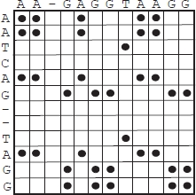
Figure 6.4. Dot matrix representing the alignment in Figure 6.1
In general, alignment problems can be divided into two categories: global and local. When looking for a global alignment, the problem consists of aligning two sequences over their entire length. In local alignment, one discards portions of the sequences that do not share any homology. Most alignment methods are global, leaving it up to the user to decide on the portion of sequences to be incorporated in the alignment.
Formally, the global pairwise alignment problem can be stated as follows: given symmetric costs γ(a, b) for replacing character a with character b and costs γ(a, −) for deleting or inserting character a, find a minimum cost set of character operations that transforms s into t. In the case of genomic strings, the costs are specified by substitution matrices which score the likelihood of specific letter mutations, deletions and insertions. An alignment A of two sequences s and t is a bi-dimensional array containing the gapped input sequences in rows. The total cost of A is computed by totalling the costs for the pairs of characters in corresponding positions. An optimal alignment A∗ of s and t is an alignment corresponding to the minimum total cost ![]() (s, t), also called the edit distance of s and t. The next section is devoted to the description of the most popular exact pairwise alignment method.
(s, t), also called the edit distance of s and t. The next section is devoted to the description of the most popular exact pairwise alignment method.
6.2.1. Smith and Waterman’s algorithm
Smith and Waterman’s algorithm is a well-known dynamic programming approach capable of finding the optimal local alignment of two strings considering a predefined scoring system that includes a substitution matrix and a gap-scoring scheme. Scores consider matches, mismatches and substitutions or insertions/deletions.
Given two strings s = s1s2 · · · sn and t = t1t2 · · · tm, the similarity S(si, tj) between sequence elements si and tj is defined and deletions of length k are given a weight Wk. For each 0 ≤ i ≤ n and 0 ≤ j ≤ m, let Hij be the optimal objective function corresponding to the subproblem of aligning subsequences ending in si and in tj, respectively. There are (n + 1) + (m + 1) elementary subproblems, whose optimal objective function value can be obtained as follows:
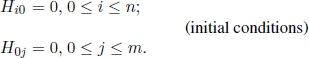
Then, for each 1 ≤ i ≤ n and for each 1 ≤ j ≤ m, the optimal objective function value Hij of the remaining n × m subproblems are recursively computed by the following recurrence equation:
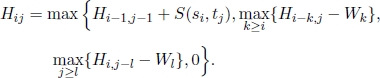
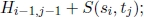
This recurrence equation considers all the possibilities for ending the subsequences at any si and any tj. The following three cases may occur:
- 1) case 1: si and tj are associated. Then, the similarity is
- 2) case 2: si is at the end of a deletion of length k. Then, the similarity is

- 3) case 3: tj is at the end of a deletion of length l. Then, the similarity is

Moreover, in recurrence equation [6.2], a “0” is included to avoid the computation of negative similarity, indicating no similarity up to si and tj. In cases where S(si, tj) ≥ 0, for all 1 ≤ i ≤ n and 1 ≤ j ≤ m, “0” does not need to be included.
An algorithm based on recurrence equation [6.2] and initial conditions [6.1] can be formulated. Moreover, we can prove that its worst case computational complexity is linear in relation to the number of subproblems to be solved, i.e. O(n × m).
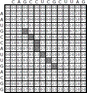
Figure 6.5. Matrix H generated by the application of Smith and Waterman’s algorithm to strings s = A A U G C C A U U G A C G G and t = C A G C C U C G C U U A G
The optimal solution computed by the dynamic programming algorithm is obtained by analyzing the matrix H. First, the maximum value in H must be located. Then, the other matrix elements leading to this maximum value are identified sequentially through a backtrack procedure ending with a “0” element in H, in this way producing the pair of subsequences and the corresponding optimal alignment. Smith and Waterman, described in their article how their algorithm applies to optimal alignment of the two sequences s = A A U G C C A U U G A C G G and t = C A G C C U C G C U U A G. In this example, relying on an a priori statistical basis, the parameter values have been set as follows:
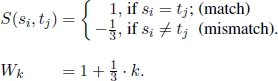
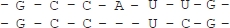
Figure 6.6. The alignment obtained for the simple example in Figure 6.5
The resulting matrix H is reported in Figure 6.5. The matrix elements in gray cells indicate the backtrack path from the element with maximum value, i.e. the backtracking starting point. The alignment obtained is shown in Figure 6.6.
6.3. The multiple alignment problem
The problem of aligning a set {s1, s2, … , sk} of k sequences is a generalization of the pairwise alignment problem and is called the multiple alignment problem. Contrary to the case of only two sequences, this problem is computationally intractable. One of the most important measures of multiple alignment quality considers an alignment as in matrix A with the input sequences (possibly extended by gaps) in the rows. Therefore, it is required that all extended sequences have the same length, which can be achieved by conveniently adding gaps. The Sum-Of-Pairs (SP) score of an alignment A, which is denoted by SP(A), is computed by adding the costs of symbols matched up at the same positions across all pairs in the sequences. Formally, the SP score of an alignment A is given by:
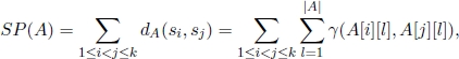
where |A| is the alignment length, i.e. its number of columns. The goal is to find an alignment that minimizes the SP score.
The computational intractability of the multiple alignment problem was proven in 1994 by Wang and Jiang [WAN 94]. A generalization of Smith and Waterman’s dynamic programming algorithm has exponential computational complexity given by O(2klk) and therefore it cannot be used to solve even small problems. In 2000, Kececioglu et al. [KEC 00] proposed an alternative and more effective method based on the maximum weight trace problem, which was introduced by Kececioglu [KEC 93] as a different optimization problem that generalizes the SP objective function score. A trace has a graph theoretic definition, but in the following we will provide a definition tailored to alignment problems. Let us suppose that k sequences have to be aligned that have o1, o2, … , ok elements, respectively. A complete k-partite graph1 G = (V, E) can be defined, where ![]() (for each i = 1, 2, … , k, Vi = {vi1, vi2, … ,
(for each i = 1, 2, … , k, Vi = {vi1, vi2, … , ![]() } is the subset of vertices of level i) and E = ∪1≤i<j≤kVi × Vj is the set of edges called lines. A line [i, j] ∈ E is realized by an alignment A if i and j are put in the same column of A and a trace, T, is a set of lines where there is an alignment AT that realizes all the lines in T. Given weights wij associated with the lines [i, j] ∈ E, the maximum weight trace problem (MWT) finds a trace T∗ with maximum total weight.
} is the subset of vertices of level i) and E = ∪1≤i<j≤kVi × Vj is the set of edges called lines. A line [i, j] ∈ E is realized by an alignment A if i and j are put in the same column of A and a trace, T, is a set of lines where there is an alignment AT that realizes all the lines in T. Given weights wij associated with the lines [i, j] ∈ E, the maximum weight trace problem (MWT) finds a trace T∗ with maximum total weight.
Recall that a cycle in a graph G = (V, E) is a sequence of vertices [v1, v2, … , vm] such that m ≥ 1, [vi, vi+1] ∈ E for i = 1, … , m − 1, v1 = vm and except for the first and the last vertex there are no repeated vertices. Moreover, a directed mixed cycle is one containing both directed arcs (elements of ![]() as defined below) and undirected edges (lines of T), in which the arcs are crossed according to their orientation, while the edges can be crossed in either direction. Let
as defined below) and undirected edges (lines of T), in which the arcs are crossed according to their orientation, while the edges can be crossed in either direction. Let ![]() 1 ≤ h < r ≤ oi} be the set of directed arcs connecting each element vir (i = 1, … , k) to the elements that are behind vir in sequence si. Kececioglu et al. [REI 97] have shown that a trace, T, must satisfy the following proposition:
1 ≤ h < r ≤ oi} be the set of directed arcs connecting each element vir (i = 1, … , k) to the elements that are behind vir in sequence si. Kececioglu et al. [REI 97] have shown that a trace, T, must satisfy the following proposition:
The property of trace T stated in proposition 6.1 is important since it has been used to formulate the MWT problem mathematically. In fact, by defining a Boolean variable xij for each line [i, j] ∈ E, the problem admits the following 0/1 integer programming formulation:
subject to:
Mixed-cycle inequality constraints [6.5] have been used by Kececioglu et al., who in [KEC 00] proposed an branch and cut algorithm. A branch and cut solution framework belongs to the family of B&B algorithms. It combines a B&B strategy with ideas from cutting planes. The first approach to find in an optimal alignment for a set of 15 proteins of about 300 amino acids was proposed by Kececioglu et al. However, it has been shown experimentally that it is not suitable for aligning sequences longer than a few hundred characters. Given the high computational complexity of multiple sequence alignment problems, several polynomial time approximation and heuristic methods have been designed to deal with long sequences and proposed in the literature. In the operations research community, an approximation method finds a possibly suboptimal solution providing an approximation-guarantee on the quality of the solution found. An algorithm Alg for a minimization problem is said to be an approximation algorithm if the worst solution returned by Alg is no greater than ϵ times the best solution, for ϵ > 1. In this case, ϵ is called the approximation guarantee of the proposed algorithm. Such approximation algorithms are important for intractable combinatorial optimization problems, since they are in a sense the best that can be done to guarantee the quality of the solution returned. A vast literature on approximation algorithms has been developed in the last decade and good starting points are [HOC 96] and [VAZ 01]. Nevertheless, sometimes it is preferable to approach and solve the problem heuristically, especially in the presence of large-scale problems. A heuristic approach finds a suboptimal solution whose quality can only be verified experimentally and, therefore, in general it is meaningful to apply it to optimization problems that are too complicated to be approximated. One of the most effective approximation methods for multiple alignment problems was devised by Gusfield [GUS 93] who proposed an iterative technique that progressively builds an alignment by considering one sequence at a time. It starts by building a star2 with a node for each of the k sequences. One of these nodes is selected as the center. The procedure, uses the tree as a guide for aligning the input sequences. With sc, c ∈ {1, … , k} is the sequence selected as the center of the star, Gusfield’s algorithm first computes k − 1 pairwise alignments Ai, one for each sequence si, i ≠ c, aligned with sc such that each Ai corresponds to the edit distance between the pair (si,sc). The k − 1 alignments can then be merged into a single alignment A(c), by putting two characters aligned with the same character of sc in the same column. Note that, in A(c) each sequence si remains optimally aligned with sc, i.e.
Therefore, it can be written that:
neglecting the specific alignment the edit distance d refers to. Moreover, by assuming that the cost function γ is a metric over the alphabet Σ, the distance is a metric defined over the set of sequences and, therefore, the triangle of inequality holds, i.e.
Let I be a generic multiple sequence alignment problem and let ![]() and
and ![]() be the optimal objective function value and the objective function value corresponding to the suboptimal solution found by Gusfield’s algorithm. In [GUS 93] Gusfield proved that
be the optimal objective function value and the objective function value corresponding to the suboptimal solution found by Gusfield’s algorithm. In [GUS 93] Gusfield proved that ![]() for any instance I. In 1999, Wu et al. [WU 99] generalized Gusfield’s method to use any tree and not only stars, preserving an approximation guarantee of 2.
for any instance I. In 1999, Wu et al. [WU 99] generalized Gusfield’s method to use any tree and not only stars, preserving an approximation guarantee of 2.
Given the computational intractability of the multiple alignment problem, to obtain good suboptimal solutions within a realistic and acceptable amount of time it was also necessary to design efficient heuristics and metaheuristics to cope with the rapid increase in the availability of biological sequence data.
6.3.1. Heuristics for the multiple alignment problem
One of the first heuristic strategies for performing multiple alignment is the progressive technique that builds up an alignment by performing a series of pairwise alignments on successively less closely related sequences. The most popular progressive method are known as Clustal [HIG 88] and its weighted variant ClustalW [THO 94]. Efficient implementations can be accessed and used via several web portals, such as GenomeNet3 and EMBNet4. ClustalW performs three main steps: 1) alignment scores are used to build a distance matrix by taking the divergence of the sequences into account; 2) from the distance matrix, a guide (phylogenetic) tree is built that has branches of different lengths proportional to the estimated divergence along each branch; 3) progressive alignment of the sequences is done by following the order of branches. Although ClustalW is among the most widely used algorithm, it suffers from its greediness and its performance depends strongly on the quality of the initial alignment. To overcome this drawback, an alternative progressive alignment method called T-Coffee [NOT 00] (Tree-based Consistency Objective Function for alignment Evaluation), has been designed. T-Coffee is also a greedy algorithm, but it is capable of finding more accurate solutions than ClustalW because it uses information from all of the sequences during each alignment step, not just those being aligned at the current stage.
Another line of research concerned with the reduction of negative effects of the shortcomings of progressive methods has led to the design of the so-called “iterative” approaches. The reason behind the choice of name lies in their characteristic of repeatedly realigning the initial sequences as well as adding new sequences to the growing multiple alignment. Progressive methods are strongly dependent on the quality of the initial alignment, because those alignments are always incorporated into the final solution. Iterative methods in contrast, can return to previously calculated pairwise alignments. Although in the scientific literature, a number of iterative methods has been proposed, implemented and made available in software packages, reviews and surveys [EDG 06, HIR 95, LEC 01] do not claim that there is one that always outperforms the competitors. The software package PRRN/PRRP, based on Gotoh’s algorithm [GOT 96], applies a greedy hill-climbing algorithm to optimize its multiple sequence alignment score and iteratively corrects alignment weights. CHAOS/DIALIGN is an alternative suite, based on the method proposed by Brudno et al. [BRU 03], that uses fast local alignments as anchor points for a slower global alignment procedure. Another iteration-based method is called MUSCLE (Multiple Sequence alignment by Log-Expectation). Proposed by Edgar in 2004 [EDG 04a, EDG 04b], it improves on progressive methods with a more accurate measure of distance.
Besides MUSCLE, there is ProbCons which is based on a technique that uses a pair-hidden Markov model and has been proposed by Wallace et al. in 2005 [WAL 05]. ProbCons introduces the notion of probabilistic consistency, a novel scoring function for multiple sequence comparisons. The use of this scoring function allows us to restrain and, therefore, cut down errors made at early stages of the alignment that not only propagate to the final alignment but also increase the likelihood of misalignment due to incorrect conservation signals.
6.3.2. Metaheuristics for the multiple alignment problem
One basic interesting question regarding multiple alignment problems is whether sophisticated metaheuristic techniques can solve large-scale molecular biology problems efficiently. For the general multiple alignment problem, besides a pioneering GA proposed by Notredame and Higgins [NOT 96], a Tabu search proposed by Riaz et al. [RIA 04], a SA proposed by Qi-wen Dong et al. [DON 06] and a hybrid ant colony proposed by Chen et al., [CHE 06], more effort has been put into this line of research recently.
6.3.2.1. Genetic algorithms
A GA is a stochastic local search procedure proposed by Holland in 1975 [HOL 75] whose main characteristic is to simulate the natural evolutionary process of species. As with any heuristic and metaheuristic approach, this type of evolutionary technique is not guaranteed to find an optimal solution. Nevertheless, in many research papers and text books (see [EIB 91, GOL 89, GOL 87]) the authors define the evolutionary process as a Markov chain and find conditions implying that there is a high probability evolution is optimum (provided infinite time or space).
Competition among individuals results in the survival and reproduction of the fittest individuals. This is a natural phenomenon called the survival of the fittest: the genes of the fittest survive, while the genes of weaker individuals perish. The reproduction process generates diversity in the gene pool. Evolution is initiated when the genetic material (chromosomes) from two (or more) parents recombines during reproduction. The exchange of genetic material among chromosomes is called crossover and can generate good combinations of genes for better individuals. Another natural phenomenon called mutation introduces new genetic material. Repeated selection, mutation and crossover causes continuous evolution of the gene pool and the generation of individuals that survive better in a competitive environment. In complete analogy with nature, once each possible point in the search space of the problem is encoded by means of a suitable representation, a GA transforms into a population of individual solutions, each with an associated fitness (or objective function value), into a new generation. By applying genetic operators, such as crossover and mutation [KOZ 92, KOZ 99], a GA successively tries to produce better approximations of the solution. At each iteration, a new generation of approximations is created by the process of selection and reproduction.
In solving a given optimization problem ![]() , a GA passes through the following basic steps:
, a GA passes through the following basic steps:
- 1) randomly create an initial population P(0) of individuals, i.e. solutions for
 ;
; - 2) assign a fitness value to each individual using the fitness function;
- 3) iteratively perform the following substeps on the current generation of the population until the termination criterion has been satisfied:
- a) select parents to mate,
- b) create children from the selected parents by crossover and mutation,
- c) evaluate the individual fitness of the offspring,
- d) identify the best individual so far for this iteration of the GA,
- e) replace worst ranked individuals with offspring.
Next, we describe how the above principles were tailored to produce a GA for the multiple alignment problem.
6.3.2.1.1. Representation and initial population
The population is represented as an array of sequences where each sequence is encoded as an array of characters over the alphabet considered. The symbol “-” refers to a gap in the alignment which represents the insertion or deletion of an amino acid residue.
6.3.2.1.2. Evaluation function
The association of each individual with a fitness value is done through the fitness function SP score, as defined in equation [6.3].
6.3.2.1.3. Parent selection
Pairs of individuals are randomly selected. Therefore, probability each individual is selected is proportional to its fitness function value: the fitter the individual, the more likely it will be chosen. Once pairs of individuals are randomly selected, clones are obtained which may then be subjected to genetic operators, such as mutation or recombination.
6.3.2.1.4. Genetic operators
Genetic operators aim to explore new regions of feasible solutions:
- – Crossover: the crossover operator uses point-to-point crossover where the operator takes two alignment sequences from the population and randomly selects a fully matched (no gap) column. After crossover, the offspring are evaluated. The fittest offspring will survive in the next iteration.
- – Mutation: the mutation operator picks a random amino acid from a randomly chosen row (sequence) in the alignment and checks whether one of its neighbors has a gap. If this is the case, the algorithm swaps (2-opt) the selected amino acid with a neighboring gap. If both neighbors are gaps, one of them will be picked randomly.
6.3.2.1.5. Replacement
This module replaces individuals that have lower fitness function values and inserts new offspring in the next population.
In 2012, Naznin et al. [NAZ 12] proposed GAPAM, an alternative progressive alignment method that applies a GA. One of the innovative aspects of this algorithm compared to the state-of-the-art is the generation of the initial population. The authors introduced two new mechanisms for this task: the first mechanism generates guide trees with randomly-selected sequences and the second one shuffles the sequences within these trees. The population size has been set to 100 individuals and in each generation, to generate a child population of 100 individuals, the following three genetic operators have been used:
- – Single-point crossover: one parent is selected from the top 50% individuals and another from the bottom 50%. The single of point crossover initially randomly selects a column position. The parent with the better score is then divided vertically at that column. The second parent is also divided into two pieces in such a way that each piece has the same number of elements as the first parent. The pieces of the two parents are then exchanged and merged together to generate two new individuals and the better new individual is considered the child.
- – Multiple-point crossovers: as in single-point crossover, one parent is selected from the top 50% of individuals and another from the bottom 50%. Unlike single-point crossover, multiple-point crossover divides each parent into three pieces that are then exchanged and merged together to generate two new individuals. The better new individual is considered the child.
To cut the first piece, the scores of the first 25% of columns for both parents are compared and the parent with the better score is divided vertically at that column, while the other parent is divided using the mechanism introduced in the single-point crossover. To create another piece and obtain three pieces for each parent, the authors applied the same idea but considered the last 25% of columns. To complete the crossover, the middle pieces are exchanged and all three pieces merged together to generate two new individuals.
- – Mutation: one individual is randomly selected from the current generation. From the individual selected, the distance between sequences is calculated and stored in a distance table. Taking into account the distance calculated a new guide tree is constructed where the sequence numbers are shuffled to find a better guide tree and the solution is considered a mutated child.
To test the performance of their algorithm, Naznin et al. compared it with existing methods, such as PRRP and different versions of Clustal, as well as the other GA-based algorithm. The experimental results showed that GAPAM achieved better solutions than the others in most cases and also revealed that the overall performance of the proposed method outperformed the other methods mentioned above.
6.3.2.2. Simulated annealing
SA is commonly said to be the oldest among the metaheuristic frameworks and one of the first algorithms that had an explicit strategy to escape the local minima. It allows moves resulting in solutions of worse quality than the current solution (uphill moves) in order to move outside local minima (see section 1.2.5 for an introduction to SA). In 2004, Kleinjung et al. [KLE 04] proposed a contact-based sequence alignment method that uses the structural information from side-chain contacts and alignment scores provided by CAO (Contact Accepted mutatiOn) substitution matrices. CAO matrices describe the probability of mutation of side-chain contacts within a protein and, therefore, they combine sequence and structure information into a single score. With alignment scores provided by the CAO, we have an approximate dynamic programming algorithm for protein sequence alignment that works assuming that the distance between the residues in contact during evolution has been conserved. Since this assumption is not suitable for insertion/deletion events during evolution, Qi-wen Dong et al. [DON 06] designed a contact-based simulated annealing alignment method that solves the problem without any restriction. The innovative aspect of this method lies in the introduction of a new parameter called contact-penalty. This parameter was introduced to efficiently and better manage the scenario where contact in the template sequence is aligned with gaps in the query sequence. In fact, when there are gaps in the contact pair, the total score of an alignment is decreased by a fixed contact-penalty. In the contact-based sequence alignment, as proposed by Kleinjung et al., there were no gaps in the contact pair due to the assumption that the distance between the residues in contact has been conserved.
6.3.2.3. Ant colony optimization
As outlined in more detail in section 1.2.1, ACO algorithms are metaheuristics that are inspired by the shortest path-finding behavior of natural ant colonies. In 2006, Chen et al. [CHE 06] designed a hybrid ACO algorithm with a divide and conquer approach for the multiple sequence alignment problem. The basic idea of this algorithm is to divide the set of sequences into several sections. The division is carried out via an ACO method by bisecting the sequences vertically and recursively. The recursive procedure ends when the length of all the sections obtained is equal to one, and hence the result of alignment is obtained. During the division phase, the proposed ant colony algorithm bisects the sequence set iteratively at approximately optimum cut-off points. Each ant searches for a set of cutting points by starting from the midpoint of a sequence and moving along the other sequences to choose the matching characters.
Let {s0, … , sN−1} be the input set of N sequences. An artificial ant starts from a randomly-selected character around the middle position of s0. Let s0[m0] be such character, where ![]() and δ is the scope of the ants search in s0. The ant selects one character from or inserts a gap into the middle part of sequences s1, … , sN−1 matching s0[0]. Furthermore, from the remaining sequences si, i = 1, … , N − 1, the ant selects a character si[j] with a probability determined by the matching score with s0[m0], the deviation of its location from the middle position of si which is given by
and δ is the scope of the ants search in s0. The ant selects one character from or inserts a gap into the middle part of sequences s1, … , sN−1 matching s0[0]. Furthermore, from the remaining sequences si, i = 1, … , N − 1, the ant selects a character si[j] with a probability determined by the matching score with s0[m0], the deviation of its location from the middle position of si which is given by ![]() and pheromone on the logical edge between si[j] and s0[m0]. The ant might select an empty character corresponding to the insertion of a gap into the sequence in the alignment. The other ants select their path in the same manner, but start from different sequences. In general, the i-th ant starts from si and successively goes through sequences si+1, … , sn−1. Once is sn−1, reached it continues going through s0, … , si−1 to complete the path. At the end of each iteration, the algorithm calculates the fitness of the solutions constructed and updates the pheromone on the logical edges accordingly.
and pheromone on the logical edge between si[j] and s0[m0]. The ant might select an empty character corresponding to the insertion of a gap into the sequence in the alignment. The other ants select their path in the same manner, but start from different sequences. In general, the i-th ant starts from si and successively goes through sequences si+1, … , sn−1. Once is sn−1, reached it continues going through s0, … , si−1 to complete the path. At the end of each iteration, the algorithm calculates the fitness of the solutions constructed and updates the pheromone on the logical edges accordingly.
In 2008, Lee et al. [LEE 08] presented a hybrid ACO algorithm to enhance the performance of a GA. In the proposed algorithm (GA-ACO), the GA is applied to provide the diversity of alignments, while ACO is performed to improve the solution generated by the GA. The initial population is randomly generated. The innovative aspect of the GA component of this hybrid approach lies in the introduction of three new crossover operators: the singlepoint operator, the recombinematchcolumn operator and the uniformexchangeblock operator. By exchanging information in parent alignments, singlepoint produces two offspring. Parent 1 is cut at randomly chosen positions and parent 2 is cut at the same ordered base position for each sequence. The remaining parts of both parents are exchanged to keep the original sequence base order, if there is a single cutting point in both parent alignments. Extra spaces may be inserted into the junction points. The recombinematchcolumn operator generates an offspring with match columns by swapping blocks and inserting spaces into the junction points, while uniformexchangeblock maps the match columns that are consistent in parent alignments. Match columns are consistent if they contain the same ordered base. Two consistent match columns are randomly selected as the two cutting points and then blocks can be directly swapped between two consistent match columns. The ACO component is embedded into GA as local search to improve poorly aligned regions.
6.3.2.4. Particle swarm optimization and Hidden Markov Models
A Hidden Markov Model (HMM) consists of a set of q states (S1, … , Sq). In the case of multiple sequence alignment, in [SUN 14], Sun et al. divided them into three groups: match (M), insert (I) and delete (D). As in any HMM: 1) two special states are defined: the begin state and the end state; 2) states are connected to each other by transition probabilities. Match and insert states emit an observable symbol (i.e. a character from the alphabet Σ) with a given probability, while the delete states do not emit observable symbols and are, therefore, called silent states. From the initial state and until the end state is not reached, the HMM generates sequences, i.e. strings of observable symbols, by making non-deterministic walks that randomly go from one state to another according to the transition probabilities. In the case of multiple sequence alignment, the sequence of observable symbols is given in the form of an unaligned sequence and the target is to find a path generating the best alignment. For a given sequence s and a HMM, a learning phase must be performed whose objective is to estimate the parameters (transition and emission probabilities). Typically, this learning task is performed by either the Baum-Welch technique, which is based on statistical re-estimation formulas, or by random search methods such as SA. In [SUN 14], Sun et al. proposed a population-based optimization (PSO) technique inspired by the collective behavior of social organisms [ENG 05, KEN 04, CLE 06, KEN 95, JOR 15]. In a (PSO) with L particles, each particle i, i = 1, … , L, represents a potential solution to the problem to be solved in a D-dimensional space. At any iteration k of the PSO, three D-dimensional vectors are associated with each particle: its current position Xi,k, its velocity Vi,k and its best position Pi,k, i.e. the position with the best objective function value or fitness value so far. A global best position vector Gk is also kept, which is defined as the position of the best particle from among all the particles in the population. For HMM learning in multiple sequence alignment, the position of a particle is composed by the parameters of the HMM, i.e. each component of the position vector is a parameter of the HMM; each component of the velocity vector represents the variation of the corresponding parameter during HMM training.
Recently, Lalwani et al. [LAL 15] proposed a two-level particle swarm optimization approach. At the first level, the particle swam optimization maximizes the matched columns, while in the second one it maximizes pairwise similarities to the best solutions found in the first level.
6.3.2.5. Tabu search
A Tabu search (TS) approach usually starts from an initial solution that plays the role of the current solution. Then, the algorithm explores the neighborhood of the current solution by generating some moves iteratively. As in the case of SA, the fundamental idea of a TS is to allow moves resulting in uphill moves in order to escape from local minima. Furthermore, it explicitly uses the history of the search, both to escape from local minima and to implement an explorative strategy. To avoid local optima and cycles, it uses a short-term memory, i.e. a Tabu list, that keeps track of the most recently visited solutions and forbids moves toward them. The length l of the Tabu list, called the Tabu tenure, controls the memory of the search process. With small Tabu tenures the search will concentrate on small areas of the search space. A large Tabu tenure forces the search process to explore larger regions, because it forbids a higher number of solutions to be revisited. The Tabu tenure can be varied during the search, leading to more robust algorithms. An example can be found in [TAI 91], where the Tabu tenure is periodically reinitialized at random from an interval [lmin, lmax].
The TS proposed by Riaz et al. in 2004 [RIA 04] has two phases. During the first phase, the search process leads iteratively to the point where the solution stabilizes, i.e. there is no improvement in the quality of solution for a specified number of iterations. Then, the second phase starts by performing intensification and diversification strategies, realized by means of elite solutions, which are the best from each iteration. The idea behind the idea of interrelating intensification and diversification strategies with elite solutions is that the neighborhoods of elite solutions likely contain attractive regions and exploring them more exhaustively may lead to better solutions than those previously encountered. Therefore, during both intensification and diversification phases, the algorithm explores the neighborhood of elite solutions. The algorithm stops when intensification and diversification strategies fail to identify new attractive regions and the best solution found is returned as the output.
As an initial solution, Riaz et al. used both an unaligned initial solution, obtained by inserting a fixed number of gaps into sequences at regular intervals and an aligned initial solution, obtained by applying a simple progressive alignment algorithm. The objective function used to measure the overall alignment quality and to evaluate candidate moves in the local search is the objective function used in T-Coffee [NOT 00]. The algorithm performs two kinds of move: single sequence moves and block moves. With single sequence moves, a patch of gap(s) of arbitrary length is moved in a randomly selected sequence while the remaining sequences in the alignment remain isolated. Block moves relocate a rectangle of gaps involving more than one sequence from one position to another in the alignment. Experimentally it has been observed that block moves are better for improving the current alignment since they involve a larger number of sequences compared with single sequence moves. Intensification strategies are based on modifying the rules that encourage the combinations of moves and solution features that have historically been good [GLO 97], while diversification strategies encourage the search process to examine unvisited regions and generate solutions that are significantly different from those already visited.
In 2015, Mehenni [MEH 15] designed an improved TS that benefits from a set of operations on the guide tree of the initial solution in order to search the neighborhood of the current solution. The guide tree carries information about the relationships between the sequences and is usually calculated on the basis of the distance matrix that is generated from the pairwise scores. The initial solution of Mehenni’s TS is represented by a tree generated by clustering the nearby sequences in a stepwise manner. At each step of sequence clustering, the sum of branch lengths is minimized by selecting the two nearest sequences/nodes and joining them. Next, the distance between the new node and the remaining ones is recalculated and this process is iterated until all sequences are joined to the root of the guide tree. Finally, the solution is obtained from the tree as follows: the pair of sequences on the lowest level are aligned, then, the entire branch containing these two sequences is aligned starting from the lowest level and progressing upward to sequences on higher levels. The SP score is used as an objective function. The innovative aspect of this metaheuristic approach lies in the local search phase, where the neighborhood of the current solution may be generated by applying one of the following four moves:
- 1) swapping move: the order of the sequences is swapped (i.e. leaves of the guide tree);
- 2) node insertion move: a certain number of nodes are inserted into the current guide tree. A node insertion can cause a sequence node to move to another location in the guide tree, therefore changing its topology. The newly obtained guide tree can be considered a neighbor of the original;
- 3) branch insertion move: a whole sub-tree (or branch) of the guide tree can be moved to another location. The topology of the resulting guide tree will change and this new tree is considered a neighbor of the current guide tree;
- 4) distance variation move: N different guide trees are produced by introducing some randomness (or noise) into the clustering algorithm used to generate the initial solution.
The TS variant that uses the branch insertion neighborhood generally outperformed the competitor strategies. No comparison is reported with other state-of-the-art algorithms.
6.3.2.6. Musical composition
In 2015, Mora-Gutiérrez et al. [MOR 15] designed two algorithms based on the method of musical composition (MMC) [MOR 12, MOR 14a]. A MMC is inspired by creativity involved in the musical composition process. The model design takes into account that musical composition can be viewed as an algorithm that is developed within a creative system, where a composer learns from his own experience and from other composers. Interactions between composers then causes the establishment of a social network. In other words, a MMC is grounded on an agent-based model of a specific social network, which is made up of a set of V nodes or agents (i.e. composers) and a set of edges E representing relationships between composers. Each composer is equipped with prior knowledge and a set of mechanisms and policies for interacting with other composers. The composers can communicate and exchange information with each other. The prior knowledge consists of a set of solutions, called tunes. The initial social network with |V | composers and a set E of links is randomly generated. For each composer i ∈ V, a set of solutions (artworks) is randomly generated. Each set generated, called a scoring matrix, represents the prior knowledge of composer i. Then, the algorithm proceeds in iterations, until a stopping criterion is satisfied. At each iteration, composers exchange information: composer i will exchange information with composer j, i ≠ j, if (i, j) ∈ E and the worst solution in the prior knowledge of composer j is better than the worst solution in the prior knowledge of composer i. If this is the case, then a new solution for composer i is generated. To evaluate the overall alignment quality, Mora-Gutiérrez et al. used two different objective functions: (1) the Euclidean distance; and (2) a multiple linear regression. The first relates the T-Coffee function, the SP-score function and the gap penalty function, while the second combines the T-Coffee function, the SP-score, the gap penalty function, the number of sequences aligned, the average length of the sequences aligned, their variation in length and Euclidean distance. Based on the experimental results, the MMC uses multiple linear regression as the objective function has been shown to have better behavior, since for 25% of the instances in the literature, it found the best alignment with respect to data.
6.4. Conclusion and future work
Sequence alignment problems are relevant to several heterogeneous scientific fields, especially in computational biology and bioinformatics, where it is fundamental to efficiently discovering the structural homologies of protein/DNA sequences and determining the functions of protein/DNA sequences to predict patients’ diseases by comparing the DNA of patients in disease discovery among others.
While the simplest alignment problem involving the alignment of two sequences (pairwise alignment) is optimally solvable in polynomial time and has been widely studied in the literature, multiple sequence alignment is a computationally intractable optimization problem and biology, computer science and operations research communities have given it less attention. An interesting, and indeed fruitful, line for future research on the multiple alignment problem includes the exploration of alternative and more sophisticated approximation and/or metaheuristic solution approaches.