
There are multiple ways to change the shape of the data. Usually, it is just projection or filtering, but there are more complex options too.
For row filters, the usual naming convention is used; that is, the node names ending with "Filter" give only a single table as a result, while the "Splitter" nodes generate two tables: one for the matches and one for the non-matching rows.
For single-column conditions, the Row Filter (and Row Splitter) node can be used to select rows based on a column value in a range, regular expression, or missing values. It is also possible to keep only these rows or filter these out. For row IDs, you can only use the regular expressions.
The rows can also be filtered by the (one-based) row index.
The Nominal Value Row Filter node gives a nice user interface when the possible values of textual columns are known at configuration time; so, you do not have to create complex regular expressions to match only those exact values.
There is a splitter, especially for numeric values, named Numeric Row Splitter. The configuration dialog allows you to specify the range's openness and gives better support for the variable handling than the Row Splitter node.
When you want to filter based on a date/time column, you should use the Extract Time Window node, which allows you to specify which time interval should be selected in the result table.
Imagine a situation where you already have a list of values that should be used as a filter for other tables; for example, you used HiLite to select certain values of a table. In this case, you can use one of this table's column to keep or remove the matching rows based on the other table's column. This can be performed by using the Reference Row Filter node. The Set Operator node is also an option to filter based on the reference table (Complement, Intersection, Exclusive-or), but in this case, you get only the selected columns and not the rest of the rows.
A very general option to filter rows is using either the Java Snippet Row Filter or the Java Snippet Row Splitter node. These are interpretations of Java (Boolean) expressions for each row, and based on these results the rows are included or excluded.
We have already introduced the HiLite Filter node in the previous chapter, which is also a row-filtering node.
If you want to split the data for training, testing, or validation, you can use the Partition node that allows you to use the usual options for this purpose (such as stratified sampling). The filtering version is named Row Sampling. If you need sampling with replacement, you should use Bootstrap Sampling.
The Equal Size Sampling node tries to find a subset of rows that satisfies the condition of each value being represented (approximately or exactly) the same number of times as a given nominal column.
This node might not be so easy to find; it is named Concatenate or Concatenate (Optional in). These nodes can be used to have two or more (up to four) tables' content in a new one. The handling of the row IDs and the different columns should be specified.
If the data you want to add is just the empty rows with the specified columns, Add Empty Rows will do that for you.
Sometimes too much data can be distracting, or it might cause problems during modeling and transformation. For this reason, there are nodes to reduce the number of columns. In this section, we will introduce these nodes.
The Column Filter node is the most basic option to remove columns. You can specify which columns you want to keep or remove. A similar purpose node is the Splitter node. The only difference is that both parts will be available, but in different tables.
The Reference Column Filter node helps in creating similar tables, but you can also use this to remove common columns based on a reference table.
When you create a column to represent the reason for missing values, you might need to replace the original column's missing values with that reason. For this task, the Column Merger node can be used. It has the option to keep the original columns too.
When you want to have the values from different columns in a single collection column, you should use the Create Collection Column node. It can keep the original columns, but can also remove them. You can specify if you want to get the duplicate values removed, or if they should be kept in the selected columns.
Sometimes, you don't have a prior knowledge of which columns are useful and which are not. In these cases, the dimension reduction nodes are of great help.
The Low Variance Filter node keeps the original columns unless their variance is lower than a certain threshold (you can specify the variance threshold and the columns to check). Low variance might indicate that the column is not having an active role in identifying the samples.
When you want to select the columns based on the inter-column correlation, you should use the Correlation Filter node with the Linear Correlation node. The latter can compute the correlation between the selected columns, and the filter keeps only one of the highly correlated columns (for "high", you can specify a threshold).
The Principal Component Analysis (PCA) is a well-known dimension-reduction algorithm. KNIME's implementation allows you to invert the transformation (with errors if any information was omitted). The nodes are: PCA (computes and applies transformation based on threshold or number of dimensions), PCA Compute (computes the covariance matrix and the model), PCA Apply (applies the model with the settings), PCA Inversion (inverts the transformation).
The multidimensional scaling (MDS) operation is also a dimension-reduction algorithm. To use a fixed set of points/rows, you should use the MDS Projection node, but if you want to use data points automatically, the MDS node is your choice.
When you have columns that contain too much data in a structured form, you might want them being separated to new columns. You might also need to combine one data source with another; we will describe how to do this in this section.
The Cell Splitter node can create new columns from textual columns by splitting them using a delimiter text, while the Cell Splitter By Position node creates the new columns by the specified positions (and column names). The first node is useful when you have to do simple parsing, (for example, you read a table with tabs as separator characters, but the date field also uses a separator character, such as /, or -), but the second is better when you have a well-defined description with fixed length parts (like ISBN numbers or personal IDs).
With the Regex Split node, you can do more complex parsing of the data. Each capturing group can be extracted to a column. Keep in mind that for groups that have multiple matches, such as (…)+, only the last match will be returned, not all, or the first.
The Column to Grid node is used for moving data from rows to new columns in the order of the rows. It will remove the unselected columns, because those cannot be represented in this way, but the selected ones will contain the values from rows in the new columns.
A practical task is referring to previous rows. It is not impossible to achieve this with other nodes, but the Lag Column node makes this an easy task.
Finally, you can combine two tables using the Joiner node. It can perform inner, left, right, or outer joins, based on the row keys or columns. This way you can enrich your data from other data sources (or from the same data source if there are self-references). If you would like to join two tables based on the row indices (practically combine them in a new table horizontally), you should use the Column Appender node.
GroupBy is the most versatile data shaping node, even though it looks simple. You specify certain columns that should be used to group certain rows (when the values in the selected columns are the same in two rows, they will be in the same group) and compute aggregate values for the nongroup columns. These aggregation columns can be quite complex; for example, you might retain all the values if you create a list of them (almost works like pivoting). If you want to create a simple textual summary about the values, the Unique concatenate with count node might be a nice option for this purpose. If you want to filter out the infrequent or outlier rows/groups, you can compute the necessary statistics with this node. It is worth noting that there are special statistical nodes when you do not want to group certain rows. Check the Statistics category for details. However, you can also check the Conditional Box Plot node for robust estimates.
With the Ungroup node, you can reverse the effect of GroupBy transformations by creating collection columns; for example, if you generate the group count and the values in the first step, filtering out the infrequent rows will give you a table, which can be retransformed with the Ungroup node (assuming you need only a single column).
Simpler pivoting/unpivoting can be done this way.
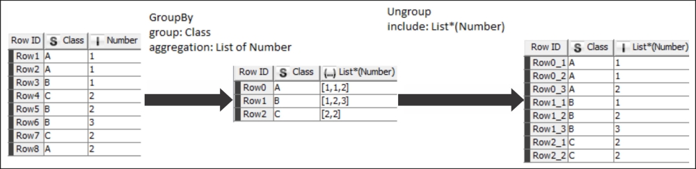
In the preceding screenshot, we start with a simple table, GroupBy using the Class column, and generate the list of values belonging to those classes, then we undo this transformation using the Ungroup node by specifying the collection column.
The Pivoting
node's basic option (when there is no actual pivoting) is the same as the GroupBy node. When you select the pivoting columns too, these columns will also act as grouping columns for their values; however, the values for group keys will not increase the number of rows, but multiply the number of columns for each aggregate option. The group totals and the whole table totals are also generated to separate the tables. The Append overall totals option has results in the Pivot totals table only.)
When you want to move the column headers to the rows and keep the values, Unpivoting will be your friend. With this node, the column names can be retrieved, and if you further process it using the Regex Split and Split Collection Column nodes, you can even reconstruct the original table to some extent.
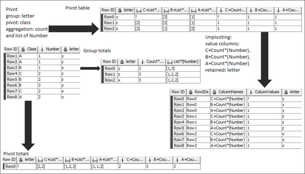
This time the initial table is a bit more complex, it has a new column, letter. The Pivot node used with the new column (letter) as grouping and the Class as pivot column. This time not just the list, but also the count of numbers are generated (the count is the most typical usage). The three output tables represent the results, while the table with the RowIDs column is the result when the Unpivoting node is used on the top result table with the count columns as values and the letter column retained.
Many modeling techniques cannot handle multinomial variables, but you can easily transform them to binomial variables for each possible value. To perform this task, you should use the One2Many node. Once you have created the model and applied it to your data, you might want to see the results according to their original values. With the Many2One node, this can be easily done if you have only one winner class label.
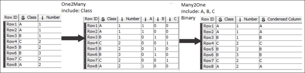
The One2Many node creates new columns with binary variables, while the Many2One can convert them back.
This section will summarize some of the options that are not so important for the data mining algorithms, but are important when you want to present the results to humans.
The Extract Column Header and Insert Column Header nodes can help you if you want to make multiple renames with a pattern in your mind. This way, you can extract the header, modify it as you want (for example, using another table's header as a reference), and insert the changed header to the result. For those places where a regular expression is suitable for automatic renames, the Column Rename (Regex) node can be used.
When a manual rename is easier, the Column Rename node is the best choice; it can even change the type of columns to more generic or compatible ones.
The Column Resorter node can do what its name suggests. You can manually select the order you would prefer, but you can also specify the alphabetical order.
Using the Sorter node, you can order your data by the values of the selected column. Other columns can also be selected to handle ties.
When you want the opposite, for example, get a random order of rows, the Shuffle node will reorder them.
The row ID, or row key, has an important role in the views, as in the tooltips, or as axis labels, where usually the row ID is used. With the RowID node, you can replace the current ID of rows based on column values, or create a column with the values of row ID. You can even test for duplication with this node by creating a row ID from that column. If there are duplicates, the node can fail or append a suffix to the generated ID depending on the settings.
When you use the row IDs to help HiLiting, the Key-Collection HiLite Translator node is useful if you have a column with a collection of strings, which are the row keys in the other table.
The Transpose node simply switches the role of rows and columns and performs the mathematical transpose function on matrices. It is not a cosmetic transformation, although it can be seldom used to get better looking results. The type of the column is the most specific type available for the original row.