4 Focus Stacking – Maximizing Depth of Field

Despite the rapid technical advances digital photography has seen in recent years, depth of field in digital images has not increased significantly. To maximize the depth of field, the smallest possible aperture is usually selected. However, this method works only up to a certain point, beyond which the laws of optics cease to improve the image: while depth of field continues to increase beyond a given aperture, the general sharpness of the resulting image begins to diminish. This effect is caused by the physical diffraction of light as it passes through the aperture opening. The f-stop at which diffraction sets in depends on the lens, its focal length, the distance between the lens and the object, and on the size of the sensor and its individual light-sensitive elements (we will discuss this topic further later on).

Maximizing depth of field is another area in which “digital optics” – i.e. computer-based digital post-processing – can lend a hand. New software can be used to merge a series of shots that were taken at differing focal distances into a single image with enhanced depth of field.

A number of programs are capable of performing this type of process. However, to keep our list of tools as short as possible (and to keep our expenses down!) we will start by using PhotoAcute, which refers to the function as “Focus Stacking”. We will also discuss the freeware program CombineZM, which, unfortunately, is only available for Windows. Another program that will be covered is Helicon Focus, an elegant and user-friendly (although rather expensive) alternative. Photoshop can also be used to perform simple focus stacking.

4.1 Why Use Focus Stacking?

Controlled depth of field is often used as a compositional tool – for example, to emphasize the face in a portrait shot by blurring the background. It is also conceivable that the photographer simply wants to use the maximum achievable depth of field, or simply more depth of field than the available equipment can provide. Depth of field is generally determined by the distance between the subject and the lens, the focal length of the lens being used, the aperture setting, and the size of the image sensor (which affects the effective focal length). This means it is possible to achieve greater depth of field when photographing an object up close with a wide-angle lens than it is with a normal lens. Some compact digital cameras can deliver more depth of field (at some apertures) than typical DSLRs. In absolute terms (disregarding the crop factor)^*, compact camera lenses are generally of a more wide-angle nature than those found on cameras with larger image sensors (APS-C or full-format 24 × 36 mm).

The size of the individual sensor elements also plays a role, and also helps to determine how far you can stop the aperture down before diffraction begins to reduce image quality.

Greater depth of field is often an advantage when shooting architectural, landscape, or macro images. When shooting macro (or micro) shots, the depth of field is always relatively small due to the unusually exaggerated relationship between subject distance and focal length. In the case of photomicrography (i.e., shots taken with a camera attached to a microscope), this distance may be no more than a fraction of a millimeter.

Under normal circumstances, you can maximize depth of field simply by setting the aperture as small as possible.^** The effectiveness of this procedure is, however, limited by the diffraction that takes place at the edges of the aperture opening. Closing the aperture down further simply reduces sharpness, and with it the usable depth of field. This is because a reduction in contrast between neighboring pixels has the effect of reducing overall image sharpness. The optimum aperture setting – known as the usable aperture – achieves the best possible compromise between depth of field and overall image resolution. It is determined by the focal length of the lens, the subject distance, the size of the image sensor, and the size of the individual sensor elements (or sensor resolution).

In the case of a digital camera with a 10-mexapixel APS-C sensor, the usable aperture is somewhere between f/9 and f/11. Higher resolutions (for the same sensor size) further reduce this value due to the even smaller distance between the individual sensor elements. Due to the small image sensors they use, most compact digital cameras have a maximum aperture setting of between f/5.6 and f/8.

Physically longer lenses (for example, macro extension rings or bellows) reduce the usable aperture value because the physical lengthening of the lens increases the effective aperture. The effective aperture is calculated based on the following formula:

Effective aperture = nominal aperture × (magnification power + 1)

The “nominal aperture” is the aperture the lens is named with. Increasing the distance between the aperture and the film (or image sensor) leads to a higher effective aperture value.

If you reduce the aperture beyond its effective point, the depth of field still increases, but overall contrast (and with it the perceived sharpness of the image) will decline.

You can find a web page for calculating effective apertures (with relation to reproduction ratios) at the address listed at [43]. Keep in mind when using this calculator, though, that the results are based on calculations made for a full-frame (24 × 36 mm) image sensor. You can read more about this topic in the article listed at [42].

If you find yourself in a situation that requires more depth of field than your current combination of camera, lens, and subject distance can provide, focus stacking is often the solution to your problem. The process hinges around taking several (otherwise identical) shots of a scene using differing focal distances. With the help of appropriate software, these images are then merged into a single, new image with maximized depth of field.

You can even conduct this type of merge “by hand” by assigning your images to individual Photoshop layers and using layer masks to isolate the areas of each image which are in sharp focus. The other problem here, is that adjusting the focal distance also slightly alters the magnification of the final image. You therefore need to scale and align each individual image accordingly. If you are only dealing with two or three shots, this technique can be quick and reliable – we will demonstrate exactly how it is done later on.

If you are handling large numbers of images, the Photoshop approach can be very cumbersome, and it is usually better to use specialized software tools. Apart from our old friend PhotoAcute, we have only found two other readily available tools that we recommend: the CombineZM freeware program[21] by Alan Haley, and the rather more expensive Helicon Focus [17], which costs about $70 for a one-year Pro license, or about $250 for an unlimited Pro license. There is also a Lite version of the software available, which is considerably less expensive and perfectly suitable for most users.

With the introduction of Photoshop CS4, Adobe has also introduced an effective focus stacking tool, which we will describe in section 4.8.

Although the focus stacking tool included with Photoshop CS4 is a big improvement, it can still be useful to use Photoshop layers to align and crop your images (as explained on page 62), before exporting them individually for merging using Helicon Focus or CombineZM^*.

4.2 What to Consider While Shooting

Taking good, sharp photos with adequate depth of field is an important initial step. You also need to differentiate between four basic types of subject distance:

“Depth of field” is often abbreviated as DOF.

1. Middle to far distance (about 15 feet to infinity)

In this type of situation, you will usually only need to shoot a single image using a relatively small aperture (large aperture value). If this does not achieve the desired depth of field, two or three shots are usually sufficient to bring the objects in both the foreground and background into focus.

2. Near to middle distance (about 2–15 feet)

Here (depending on the lens you are using and the subject), two, three, or four shots are usually sufficient.

3. Close-ups (½ inch to approximately 1 foot)

Shooting at these distances requires the use of specialized macro equipment (when using a DSLR)^* and usually between 3 and 6 shots.

4. “Real” macrophotography (from ½ inch right down to the photomicrographic level)

Here, you may have to take a large number of shots, as depth of field shrinks rapidly with increasing magnification. Here, the depth of field involved can be as little as a fraction of a millimeter.

If you are working with a DSLR, you should have a good idea of the usable aperture your camera (or camera/lens combination) provides.

Establishing the “Optimum Aperture” Using Test Shots

Here, you will simply need to experiment to find the ideal setup. To eliminate the risk of camera shake, you should take all of your test shots using a stable tripod, a remote or cable release (or a timer), and if possible, mirror lock-up. Start at around f/5.6 and take several shots, decreasing the aperture each time until you reach the limit your lens permits at the zoom setting you are using.

You can now download your test images to your computer and perform any necessary RAW conversion while taking care not to sharpen your images manually during the process. You can then compare your images (ideally at 100% magnification), and identify the aperture (to be found in the EXIF data associated with each image) at which depth of field no longer increases and contrast (and therefore perceived image sharpness) begins to decrease. This is the point at which your optimum aperture lies, and is usually found at around f/11 for an 8-megapixel APS-C camera, and at around f/9 for a 10-megapixel APS-C camera. The value should increase to approximately f/16 for an 11-megapixel full-frame camera, such as the Canon 1Ds, and should be around f/8 in the case of a 21-megapixel full-frame camera, such as the Canon EOS 1Ds Mark III.

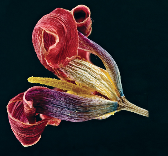
You will need to repeat these steps for various subject distances, as the reproduction ratio also plays a role in determining sharpness and depth of field. We recommend that you use a purpose-built test chart (like the one shown in figure 4-1). In order to achieve accurate results, the chart needs to be exactly parallel to the image sensor while you are making your test shots.

A good explanation of diffraction and its effects on image contrast and resolution can be found at [42].

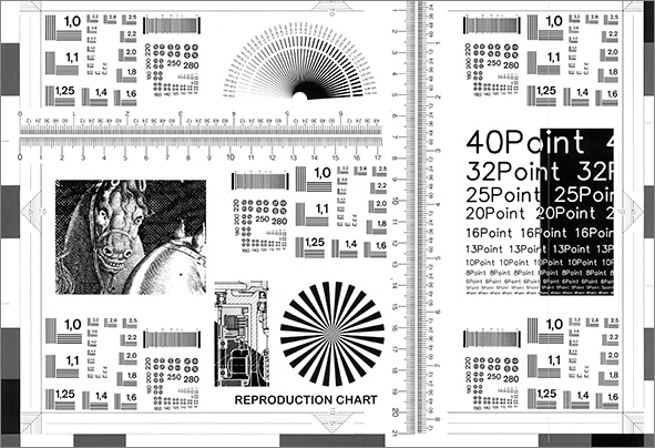
Figure 4-1: Heavily scaled down image of a test chart used to determine sharpness and the associated “optimum aperture” of a camera/lens combination.

Optimum Aperture for a Standard Print

If you are only considering the point at which diffraction effects become visible in a standard (8 × 10 inch) print, you will most likely achieve results similar to those listed in table 4-1. The table was calculated based on the following formula:

Whereby:

u	=	Circle of confusion diameter (assumed to be 0.03 mm for the 35 mm format)
λ	=	Wavelength of the light involved (550 nm is the assumed average)*
m	=	Magnification ratio

This table takes neither sensor resolution nor the size of the individual sensor elements into account. At higher resolutions, the optimum aperture value is further reduced (as demonstrated above) for as long as you use higher resolution to make larger prints.

Table 4.1: “Optimum aperture” (OA), calculated for various magnification ratios and sensor sizes
Magnification ratio:	1:2	1:1	2:1	3:1	4:1	5:1	7:1	8:1	10:1	Circle of confusion
OA Medium Format (57 × 57 mm)	49.7	37.3	24.8	18.6	14.9	12.4	9.3	8.3	6.8	0.050 mm
OA Full Format (24 × 35 mm)	29.8	22.4	14.9	11.2	8.9	7.5	5.6	5.0	4.1	0.030 mm
OA Crop Factor 1.3	22.9	17.2	11.5	8.6	6.9	5.7	4.3	3.8	3.1	0.023 mm
OA Crop Factor 1.5	19.9	14.9	9.9	7.5	6.0	5.0	3.7	3.3	2.7	0.020 mm
OA Crop Factor 1.6	18.6	14.0	9.3	7.0	5.6	4.7	3.5	3.1	2.5	0.019 mm
OA for -Format (CF = 2)	14.9	11.2	7.5	5.6	4.5	3.7	2.8	2.5	2.0	0.015 mm
OA -Sensors	7.9	6.0	4.0	3.0	2.4	2.0	–	–	–	0.008 mm
OA -Sensors	6.0	4.5	3.0	2.2	–	–	–	–	–	0.006 mm
OA -Sensors	5.0	3.7	2.5	1.9	–	–	–	–	–	0.005 mm

4.3 Shooting for Focus Stacking

As described above in the section about test shots, you will need to avoid camera shake as much as possible when shooting focus stacking sequences. This is best achieved by using a tripod, a cable (or remote) release, and, if possible, mirror lock-up. Mirror lock-up prevents vibrations caused by the mirror’s travel from being transmitted to the tripod. If you are taking true macro shots, we recommend the use of a focusing rail instead of your camera’s focusing ring (see figure 4-2 for an example). If you are using bellows, the rail is usually already built in.

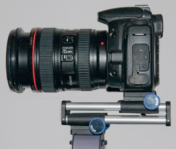
Figure 4-2: A macro focusing rail helps with precision focusing when shooting close-ups or macro photos. (The illustration shows the Novoflex “Castel-Mini”.)

When taking macro shots of nature subjects, it is useful to have a tripod that can be set up to work close to the ground. The best option here is a boom tripod like the one shown in figure 4-3.

You should also switch to manual focus in order to focus accurately, and it always an advantage to use the camera’s depth of field preview button to ascertain in advance how many shots you will need to take and where to focus for each. To begin with, we will only focus roughly, and we will fine-tune our settings later using the bellows or the focusing rail. Start with the foremost focus distances and work your way backwards.

When shooting landscapes or architectural shots, we usually use the focusing ring on the camera’s lens.

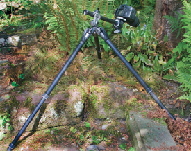
Figure 4-3: Boom tripod (here, a Gitzo “Explorer 2”).

If you are working with a cable or remote release and an SLR camera, you will often not be using the viewfinder. This can cause stray light to reach the lens through the viewfinder, making your image duller than it otherwise might be. You can avoid this problem by covering the viewfinder eyepiece. The neck straps included with some Canon DSLRs include a rubber cover specially designed for this purpose.

Your subject will, ideally, not move between shots, but minor movements can be compensated for later using appropriate software. It is also important to take your shots in rapid succession to avoid any changes in lighting that affect your results. As far as we are aware, there is currently no camera that has a focus bracketing function. Remember to adjust your focus settings in one, consistent direction – i.e., from front to back or back to front, and do not switch direction mid-sequence.

If you are shooting in JPEG or TIFF format, you should used a fixed preset white balance value in order to keep the color temperature consistent for your whole sequence. The aperture and exposure time also need to be consistent, so it is best to work in manual mode as often as possible. Most focus stacking programs (especially Photoshop) can compensate for some exposure discrepancies between shots.

The number of shots you need to take will depend on the subject, the subject distance, the lens you use, and its optimum aperture; and on your own personal standards. We recommend that you start by taking three- or four-shot sequences in order to gain some experience. Macro shots with high magnification ratios will require you to take additional shots in order to achieve high-quality results. It quickly becomes obvious when there are blurred gaps between the in-focus regions of an image; the in-focus areas of the individual shots should always overlap.

When taking close-ups using a macro lens and a focus rail, we only use the camera’s focusing ring for the first shot. All subsequent shots are focused using the focusing rail in order to avoid the changes in lens length (and the resulting change in effective aperture) that focusing a macro lens causes.^*

The focus stacking applications mentioned in this book can all handle large numbers of images in a stack, although dealing with large numbers of images in Photoshop can quickly become tiresome. It is, therefore, a good idea to take too many rather than too few shots. This way you avoid the risk of having gaps in the focus of your final image. The first step in a merge process will always be to load your images and to discard any shots that are too similar or that are not in focus.

As already mentioned, the depth of field preview button can help to ascertain exactly how much depth of field you will be able to achieve for a certain shot. Most DSLR cameras have this functionality, as do some bridge cameras. However, in instances where the aperture is small, the image in the viewfinder will quickly become dark, making it hard to evaluate depth of field. In this case, experience helps.

Preprocessing

Regardless of which program you choose to use, we recommend renaming your images so that they maintain their sequence when sorted numerically. It is also a good idea to save the images from a single focus stack in their own folder as illustrated in figure 4-4. Alternatively, some image database software (such as Apple Aperture or Adobe Lightroom) allows you to group your files into a stack.

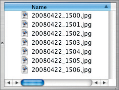
Figure 4-4: The file names you give your images should reflect the order of the stacking sequence.

Your shooting format and the program you use will determine whether you have to preprocess your images before merging. Photoshop and CombineZM cannot process RAW files, so if you shoot RAW images, the first step will be to convert the file format. CombineZM requires 8-bit images as input, but Photoshop can also handle 16-bit (per color channel) images. PhotoAcute and the Windows version of Helicon Focus can process RAW as well as 16-bit TIFF and 8-bit JPEG files. You can find out whether using RAW input files suits your purposes simply by experimenting.

Make sure you subject all your images to the same preprocessing steps (white balance, exposure compensation, vignetting, and other color and tonal corrections). We will perform all other fine-tuning, including sharpening and perspective correction, once the images have been merged.

To begin with, apply the same changes to all of your images. Most currently available RAW converters (e.g., Adobe Camera Raw, Adobe Lightroom, Apple Aperture, or Capture One) allow you to optimize the first image in a stack and then apply your settings to all subsequent images using a built-in synchronization function (as described in section 2.1 on page 16). This will give all the images in your sequence a similar (or identical) distribution of luminance and color tone.

In all other cases, export your images at the highest possible resolution to TIFF or JPEG. If you choose to shoot JPEG images directly, use the highest image quality and the lowest compression setting possible. When exporting images from a RAW converter, you should always export to TIFF, because the quantization automatically applied during JPEG conversion can spoil the merge process later on. (Quantization creates groups of pixels within single-color image areas so they can be coded more efficiently into the resulting image file.)

Should you want to publish your merged image online, or send it as an e-mail attachment, you should only perform any necessary scaling or compression on the final, merged image, not on your source images.

4.4 Focus Stacking Using Photoshop

The workflow we describe in this section may appear highly technical to some of our readers. Those who prefer to use more automated processes can skip directly to section 4.5 on page 66.

Photoshop versions up to and including CS3 do not offer an automated focus stacking tool. You can, however, still use Photoshop to perform this task manually. The required steps – loading, aligning, rotating, scaling, and merging (also called blending) – are described here in detail. The individual steps also apply to the other programs we have mentioned, although the process is automated to varying degrees in PhotoAcute, CombineZM, and Helicon Focus.

1. The first step is to load the source images. Because Photoshop cannot process RAW images directly, these will be loaded through Adobe Camera Raw into Photoshop as TIFF, PSD, or JPEG files (16-bit TIFF and PSD files are preferable).

Once loaded, the individual images should be stacked in individual layers in order of focus distance.

2. The layers are inspected individually, and any unusable images are removed by deleting or disabling the appropriate layer.

3. Align each image horizontally and vertically in order to achieve the best possible coverage. Some of the images may need to be rotated or even scaled (enlarged or shrunk). We will show you later how to automate the first three steps in Photoshop CS3 using scripts.

4. Use layer masks to suppress the areas of each image (or, in Photoshop, the layers) that are not in focus.

5. Finally, crop the image to remove any margins created by rotation and scaling, and to leave only the areas in sharp focus.

6. You can now (optionally) merge your layers into a single image layer.

Don’t let Photoshop’s complex methodology intimidate you – the program has comprehensive help files, and many of the steps described are automated in PhotoAcute, CombineZM, Helicon Focus, and more recently in Photoshop CS4.

The following example demonstrates the process. We have two source images of a street, both of which cannot encompass the necessary depth of field to show the entire scene in focus (see figures 4-4 and 4-5). Both images contain detailed elements all the way from the near foreground to the far background (or “infinity”).

Figure 4-5: This picture is sharp from the foreground up to about the middle of the view.

Figure 4-6: Here, detail from the middle distance to infinity is sharp.

The technique used in Photoshop versions up to CS2 involved opening both images and selecting (using or ) and dragging (by holding down ) the entire second image (focused towards the rear of the scene) to cover the first.

You then need to align the two images. In our example, we will only move the upper image using the tool and the arrow keys on the keyboard.

If we need to rotate and scale the result, we first need to increase the canvas size using the crop tool . Next, we activate the upper layer, select all (), and use or to activate the free transform and scaling tool. We then scale and rotate the layer until satisfactory coverage is achieved. During this last step, it is often helpful to set the layer mode to Difference (see figures 4-7 and 4-9).

Figure 4-7: Our layer palette with the blending mode “Difference” activated to check the alignment of our two layers.

As of the CS3 version, Photoshop handles most of this process using a specially developed script, which can be found under File ▸ Scripts ▸ Load Files into Stack.

In the script’s dialog box, we select all of our source files and select the option Attempt to Automatically Align Source Images (see figure 4-8). It may still be necessary to scale the images later.

As already mentioned before, the level of coverage can be made visible using the Difference blending mode. Figure 4-9 shows that we have fairly good coverage, with only slight overhang resulting from the two different focal distances.

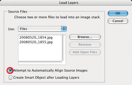
Figure 4-8: Photoshop CS3 includes a script called “Load Files into Stack”. It allows you to load several images into separate layers and to align them.

The next step involves masking the unsharp areas of the uppermost layer (or all layers if you are working with multiple images). This is fairly straightforward for our simple architectural example.

To get started, we click the layer mask icon at the bottom of the Layers palette to create a new, white layer mask, making sure this new mask is active by clicking on the layer mask icon:

Our layers palette now appears as illustrated in figure 4-10.

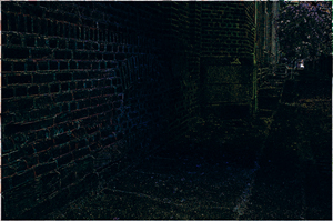
Figure 4-9: Setting the layer blending mode to “Difference” will show how well the images in two layers fit. It shows the differences between the two layers in white.

The blending effect here is obtained by applying a simple black-to-white color gradient to the layer. The section of the image covered in black will be masked and where the mask is gray, we will have a semi-transparent layer. In this case, we want to mask the unsharp parts of the upper image in order to expose the sharp elements of the image beneath.

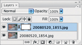
Figure 4-10: The layer palette shows our two aligned images (layers). In the upper layer the layer mask is empty and activated.

To do this, we first click on the foreground color icon in the Photoshop toolbar and press to activate black-and-white mode for the foreground and background colors. We then select the gradient tool , which is sometimes hidden behind the icon for the paintbucket tool.

To create the gradient, click on the left edge of the image and hold down the mouse button while dragging the cursor across to approximately the center of the image area, then release the mouse button. This will generate the gradient we need to create the mask, which should look something like the one shown in figure 4-11. If it doesn’t look right, simply try again. In the area where the gradient fades to gray, the masking effect will correlate to the gray scale value, allowing the image beneath to show through more where the gradient is lighter and less where it is darker.

The result of the blending process can be seen in figure 4-12, and figure 4-13 shows the corresponding layers palette.

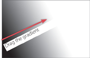
Figure 4-11: Gradient layer mask used for the upper layer (created using the gradient tool).

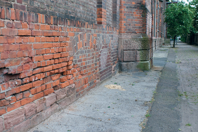
Figure 4-12: The merged image with increased depth of field.

If you are working with a more complicated scene, a large, soft brush tool is more appropriate than the gradient tool. This will allow you to work around the contours of unfocused areas and mask them accurately with black, or to expose the sharp areas under a black mask using a soft, white brush. During brush work in masks, it is important to make sure that you are working on the mask (by clicking the mask icon) and not on your original image file.

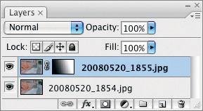
Figure 4-13: Layer palette showing the two layers used in figure 4-12.

An Example with Four Source Images

The process described above also works with more layers, and for images with varied depth of field. Our example uses the following four shots of a fern frond uncurling, whereby each shot has a different depth of field (see figure 4-14).

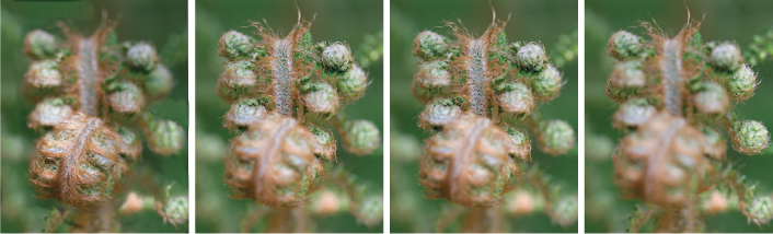
Figure 4-14: Our source images – greatly reduced.

When working with multiple images, it is a good idea to create a white layer mask for all layers except the one at the bottom of the stack. The layer palette will then look something like the one shown in figure 4-15.

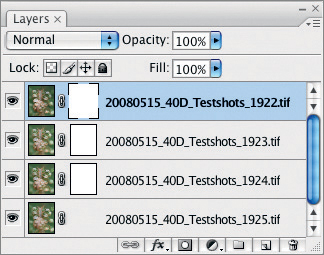
Figure 4-15: Our four source images loaded and aligned, each with its own white layer mask.

We then hide all but the uppermost layer by clicking on the eye icon next to the name of each layer in the palette. Now activate the layer mask for the top layer and mask all unsharp areas using a large, soft black brush. You can use a smaller diameter brush to work around the finer details.

The final image should look something like the one in figure 4-16, showing only the areas of the layer that are in focus, with all other layers hidden.

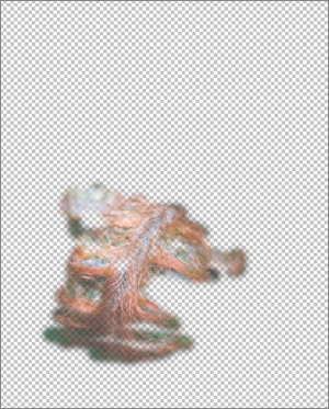
Figure 4-16: Preview with active layer mask and all other layers hidden.

Once a layer is done, move on to the one directly below it. Unhide the layer, activate its layer mask, and repeat the process of masking all the unsharp areas in black. Finally, activate the bottom layer, but here, do not perform any masking. Figure 4-17 shows the resulting layer palette, in which the individual masks are visible.

It is helpful to occasionally hide the individual layers during the masking process (by holding and clicking on the appropriate mask icon). This helps you to see if the mask is a good fit. If you have masked too much detail, you can go back and make corrections using a white brush. Zooming in and out while painting the mask also helps you to work more accurately.

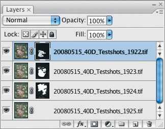
Figure 4-17: The Layers palette showing all layers and their corresponding layer masks.

Finally we applied some mild local contrast enhancement using DOP Detail Extractor (as described in section 7.1), and a little sharpening using the Photoshop USM filter to achieve the result you can see in figure 4-18.

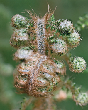
Figure 4-18: The result of our Photoshop merge process. The source images were taken using a Canon 40D with the Canon 100 mm F2.8 macro lens. The subject distance was about 14 inches. We used the camera’s built-in flash and a working aperture of f/11.

This process will possibly appear complicated and laborious, therefore the programs we will now describe will help you to achieve similar results in a simpler way. Nevertheless, with a little practice you can achieve satisfactory results fairly quickly using Photoshop. Processing our four-image example took about 20 minutes from start to finish.

In section 4.8 we will show you how to automate focus stacking processes using the new features included in Photoshop CS4.

4.5 Focus Stacking Using PhotoAcute

For this example we photographed an old Leica camera. As figure 4-19 illustrates, the depth of field in a single shot is too shallow to encompass the entire camera body and extended lens. We therefore used our Nikon D300 with a Nikon 60 mm f/2.8 macro lens set at f/9 to take five shots, each with the focal distance pushed a little further back.

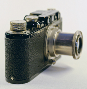
Figure 4-19: We photographed this old Leica using a Nikon D300 with a 60 mm macro lens set to f/9. Shot from close up, only a small part of the camera is in sharp focus.

We used a stable tripod, and the camera was set to Manual in order to ensure constant exposure values throughout the sequence. Autofocus was deactivated and we focused each shot manually. We used a cable release and mirror lock-up to further reduce the risk of camera shake.

We used drag & drop to load our JPEG source files from Adobe Bridge into PhotoAcute, giving us a start scenario as depicted in figure 4-20.

Because PhotoAcute has yet to offer a profile for the Nikon 60 mm macro lens we used, we chose the most similar lens (a Nikon 50 mm 1.8) from the dropdown menu (see figure 4-21 ).

A click on the Start button opens the Processing dialog box, where you can set parameters shown in figure 4-21. The most important setting is the Focus Stacking command located in dropdown menu , which tells the program to merge the images into a single image with extended depth of field.

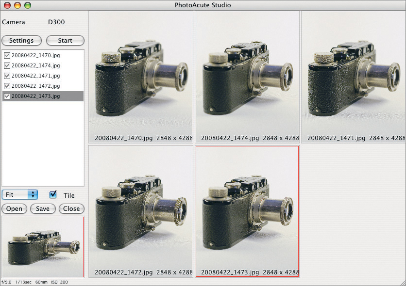
Figure 4-20: The five source images are first dragged to the open PhotoAcute window from Bridge (or whichever other image browser you are using). Don’t forget to activate your source images! PhotoAcute automatically recognized the camera type, but we had to manually select a lens similar to ours, as PhotoAcute does not yet support the actual model we used.

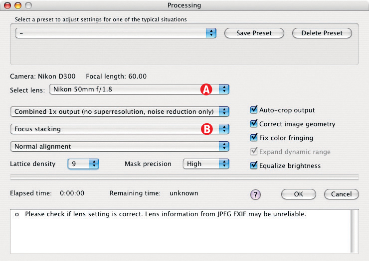
Figure 4-21: Our Focus Stacking settings: The illustration shows PhotoAcute version 2.8.

Clicking OK will start the merge process. Processing five source images will take some time, even if you are using JPEG files and (as we did) a fast, four-processor Macintosh. The result of the focus stacking run can be seen in figure 4-22.

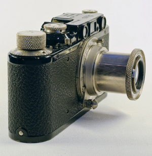
Figure 4-22: The result of our PhotoAcute process.

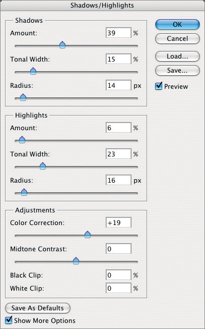
Figure 4-23: We used the Photoshop Shadows/Highlights function to brighten up the dark regions of the image.

At this point, the side of the camera closest to the viewer appears a little dark, as well as and the black metallic parts of the camera.

To brighten up these parts of the image, we used the Photoshop Shadows/Highlights tool. The settings we used are shown in figure 4-23.

In figure 4-24 we see the final image, which shows a degree of consistent sharpness that we couldn’t have achieved with our standard equipment.

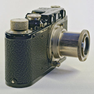
Figure 4-24: The result of merging five source shots with differing focal distances, and then lightening some shadows using the Photoshop Shadows/Highlights tool.

We then noticed the moiré effect caused by the cloth we used as a backdrop, so we decided to adjust the background using Photoshop.^*

We used Photoshop’s Gaussian Blur filter to create a soft-focus effect in the background cloth, while retaining sharpness for the camera itself. To achieve this we need to select a suitable area using Select ▸ Color Range. In the dialog box which appears (see figure 4-25), start by setting the dropdown menu Select to Sampled Colors.

Then activate the eyedropper , and click in a part of the image where the cloth is relatively bright. Use the Tolerance slider to set the camera apart from the background (it should be marked black). Details like the shadow under the camera’s lens can be corrected later on.

Then, with our selection activated, we duplicate the background layer by clicking Layer ▸ Duplicate Layer. This new layer will automatically contain a layer mask which protects the parts of the image containing the camera from being processed by the applied filters.

The layers palette will now look like the one in figure 4-26. At this point, we named the new layer Gaussian Blur.

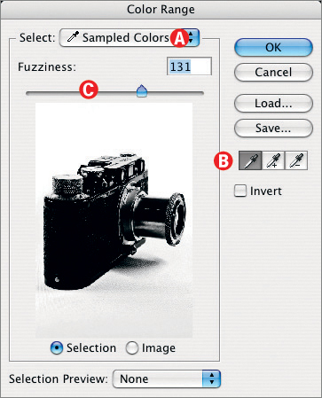
Figure 4-25: Using the Select ▸ Color Range dialog helps us to create a new layer mask for use later on.

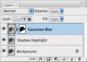
Figure 4-26: The Layers palette should look like this once you have created and activated the new layer.

We now select the desired filter via Filter ▸ Blur ▸ Gaussian Blur, select a moiré-affected area with the mouse, and use the Radius slider (see figure 4-27) to increase the filter effect until the moiré pattern is no longer visible in the preview window.

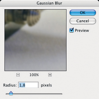
Figure 4-27: Increase the Radius value until the cloth pattern disappears.

The Preview option should be activated during this process, in order to make the effect of your adjustments visible in the entire image, and not just the preview thumbnail.

Because the layer mask wasn’t perfect, and parts of the camera and lens weren’t completely covered by it, we now click on the layer mask icon in the layers palette to reactivate the mask. We then use the brush tool (with the color set to black and sharpness set to soft) to rework the boundaries of the area which need to be excluded from the Gaussian Blur effect. As you paint into the mask, the active layer will be hidden under the black areas you create and the in-focus image in the layer behind it will become visible. We then continue to fine-tune the layer mask using black and white brushes until it fits perfectly around the camera in the image.

In addition to the unwanted cloth pattern, the image in figure 4-24 also shows a slight yellow color cast, caused by the color of the lamp used to light the scene. Ideally, we should have corrected this color cast by adjusting the white balance in a RAW converter, but we would then have had to adjust the levels for each individual source image.

We can correct the color cast using an adjustment layer, via Layer ▸ New Adjustment Layer ▸ Hue/Saturation. In the dropdown menu Edit in the resulting dialog box, we choose Yellows (see figure 4-28). We then use the eyedropper tool to select an area of the image with a relatively pronounced color cast – the upper edge of the lens barrel, for instance. We then reduce saturation using the Saturation slider until the color cast is no longer visible. In our example, this occurred at a saturation value of “-48”.

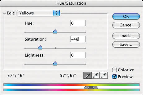
Figure 4-28: We reduced the yellow cast visible in figure 4-24 by reducing saturation for yellows.

We now select Blues from the Edit menu to correct the blue cast that is also affecting the camera lens in our image. Again, we use the activated eyedropper to select an appropriately colored area, and reduce saturation while adjusting Hue slightly towards green (see figure 4-29). At this point, the Layers palette should appear as illustrated in figure 4-30.

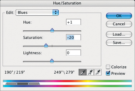
Figure 4-29: Here, we have reduced the blue cast visible along the upper edge of the camera’s lens in figure 4-24.

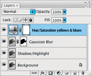
Figure 4-30: The Layers palette for the image in figure 4-31 showing all the fine-tuning layers we used.

As a final touch, we could also lighten the shadow under the camera’s lens. Here, we use a Curves (or Levels) adjustment, coupled with a mask that covers almost the entire image save for the shadow area, which remains white.

Because PhotoAcute sharpens your images automatically, you only need to apply slight additional sharpening before printing. If you plan to present your results on a monitor, online, or in a slide show, no further sharpening will be necessary. RAW source images always require more sharpening at the presentation stage, as these are generally softer than images originally shot in JPEG format.

If the program’s almost exaggerated automatic sharpening is too much for your taste, you can use the Oversharpening Protection slider to keep this effect in check. The slider can be found in the Advanced tab of the Preferences dialog (see also the description on page 35).

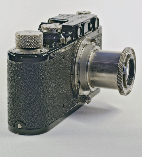
Figure 4-31: The final image. The moiré pattern in the background cloth is gone, and the yellow color cast has been neutralized.

When shooting images for advertisements (especially with flash), reflections can often cause problems in the resulting images. This type of problem can be effectively reduced using a polarizer, and flash can usually cope with the 1 ½ to 2 stops of exposure darkening that a polarizer causes. A polarizer cannot, however, reduce reflections from metal surfaces, as our example shows. Here, you can use either softer lighting, or an anti-reflective spray (available at most specialty photo stores).

4.6 Maximizing Depth of Field Using CombineZM

CombineZM is currently freeware, and is designed to work with Windows 2000 (and newer) systems. The version we used for our example can be downloaded from the link listed at [21], or via our the publisher’s link page at www.rockynook.com/tools.php. We recommend downloading the msi-version, as this is easiest to install. The installation automatically adds a program icon to the user’s desktop.

When starting CombineZM for the first time, you should go to File ▸ Set Options and increase the memory, which the program allocates for processing. We recommend allocating 1024 MB of RAM if possible. These changes will take effect after you restart the program.

CombineZM is a powerful program, and offers the user a much greater degree of control over the merging process than PhotoAcute. It can handle JPEG and TIFF files as well as a number of other formats, including BMP, PNG, and GIF. It cannot, however, process RAW or DNG files.

CombineZM is also limited to processing 8-bit images (8 bits per RGB color channel), but is, similar to PhotoAcute, also capable of more than just focus stacking. We won’t however, be addressing the program’s noise reduction or tone averaging functions at this point.

The power of CombineZM, which can also extract images from several video formats, comes at the price of increased complexity. Here, we will detail a simple application, so as not to move outside of our declared scope for this book.

CombineZM Terminology

CombineZM uses partially proprietary terminology, so we will explain the most important terms in the following sections.

The author of CombineZM provides some online help documentation, but not enough to develop a thorough understanding of the program. Most online CombineZM tutorials also lack depth. If a good manual or a comprehensive tutorial were available, the public would be able to get a lot more out of the program! Nevertheless, a good place to look for help is: http://tech.groups.yahoo.com/group/combineZ/

The individual images which are to be merged are called frames. CombineZM can load, store, and process up to 255 frames, provided your computer has enough RAM. The appropriate frames have to be loaded into the program before any processing can take place.

As previously described in the Photoshop section, the individual images (frames) are also loaded into a focus stack – in CombineZM, called simply a stack – where alignment and further processing takes place.

The processing itself is controlled by commands or combinations of commands, which are stored in macros. CombineZM provides a number of standard macros to cover most standard processing situations, but you can also write custom macros for particular combinations of commands if necessary. These macros can be found in the Macro menu, and we will be concentrating mainly on using Do Stack and Do Soft Stack.

While merging multiple frames into a single image with enhanced depth of field, CombineZM creates a special depth of field map of the process, called a depth map. The program uses the depth map to determine which parts of each source image will be used when piecing the final image together. This process is similar to the manual layer masks we used for the Photoshop-based focus stack.

CombineZM displays a macro’s progress in the Progress window. As the individual steps making up a macro can be fairly time-consuming, the progress window also displays a moving, gray progress bar for each individual step (see figure 4-34).

Sample Merge Using CombineZM

For this example, we will once again use our old Leica. We shot our source images from closer than before, and from a different angle. Here, in order to obtain sufficient depth of field, we made eight different exposures.

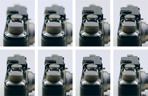
Figure 4-32: Our favorite old Leica, this time shot from a different angle using a Nikon D300 and a Nikkor 60 mm f/2.8 macro lens set to f/8.

After starting CombineZM, we use File ▸ New to load our source images, by navigating to the folder where the images are stored, and then selecting them and loading them using the - or keystroke.

In the File dialogs in CombineZM and all the other programs we have described, the key can be used to select multiple files which are grouped together, and the key can be used to select multiple files which are not listed consecutively.

During the loading process (and all other processing steps), CombineZM temporarily closes the main window and displays a progress window instead. As previously mentioned, you should give your images file names that adhere to the desired order of your stack – from front to back, or vice versa.

After the loading is complete, the main window will reappear, displaying the bottom image of our stack (figure 4-33).

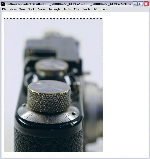
Figure 4-33: CombineZM’s main window after loading the source images into the stack. The first frame in the stack will be displayed.

At this point you can once more inspect your images individually. Press the function key to open a window displaying all the images in the stack. Select the image you want to view and click OK – CombineZM will then display that image in the main window.

Next, we begin the focus stacking process by starting the Do Stack macro, which is located in the Macro menu. The program will now display the progress of each individual macro step in the CombineZM Progress window (see figure 4-34).

If you are working with large numbers of images or large image files, this process can take some time. The main window will, however, eventually reappear, displaying the resulting new, stacked image (figure 4-35).

You can pull up the progress window at any time by pressing , in order to review the steps that have already been completed, to check the parameters that have been set, or to check for any warnings or error messages.

Clicking the Minimize button at the bottom left of the window does just that, and the progress window will disappear.

If the results are to our satisfaction, we can save our new image using the command File ▸ Save Frame/Image As.

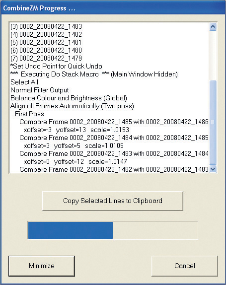
Figure 4-34: CombineZM hides the main program window, and instead displays this progress window during processing. It shows the progress of the individual steps being performed.

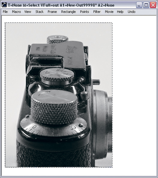
Figure 4-35: Once the macro has been executed, CombineZM closes the progress window, reverts to the main window, and displays the resulting merged image.

Here, we can specify the format the image is saved to. If you think your image will need further processing, then TIFF is the best choice. Figure 4-36 shows the formats the program offers.

If, on the other hand, the merged image doesn’t exactly match your expectations, the program offers various options for making a second attempt. The first option is to use the command Do Soft Stack instead of Do Stack.

It often helps the process to succeed if you select a reference image from the middle of your sequence, or at least an image in which the most important part of the subject is in focus. You can then use this reference image as your starting point for processing.

If you haven’t managed to achieve satisfactory results after two or three attempts, it can help to simply close the program and start again from scratch. This rather brutal approach has helped us to get better results on a number of occasions.

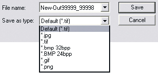
Figure 4-36: CombineZM offers several output formats for your merged images.

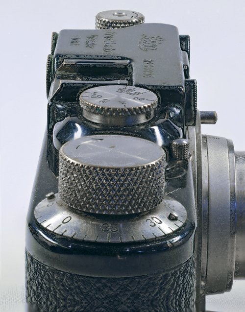
Figure 4-37: Result of our CombineZM focus stacking process, using eight source images, the standard “Do Stack” macro, and the program’s default settings.

In our example, the first merged image turned out fine. As with our previous example (see page 70), we lightened the shadows using the Photoshop Shadows/Highlights tool, and we removed the slight yellow color cast present in the source images using a Hue/Saturation adjustment layer. The final result can be seen in figure 4-37.

All of the multishot programs we use require a substantial amount of processor power and RAM. It has happened – while processing many and/or large images in CombineZM – that our Windows system simply ran out of memory or swap space and froze.^* If this happens to you, it might be necessary to scale your images to a smaller size before attempting to merge them.

That concludes our whistle-stop tour of simple focus stacking methodology using CombineZM. CZM is, however, capable of much more than that, and we encourage you to go ahead and experiment. Amongst the other functions the program offers, you can start by manually aligning the images in your stack before merging, using Stacks ▸ Site and Alignment. The program also applies masks to the individual frames in a stack to determine which parts of each frame will appear in the final merged image. These so-called depth maps can be saved separately, as can the rectangles for the individual frames in the stack, so you can use the same reference points later for a different merge.

CombineZM also enables the user to create custom macros, to load macros written by third parties, and to customize the macros provided with the program. This is easy to do – simply go to Macro ▸ Edit and select the macro you want to modify. This will open the selected macro in a macro editor, where you can, for example, build in new filters or entire processing steps.

In addition to the dialog-based version of CombineZM, there is also a batch-oriented version called CZBatch available. This version is used for merging multiple stacks into images with enhanced depth of field. To use the batch version of the program, you should save each stack that you wish to merge in a separate folder, and save these folders in a special batch folder.

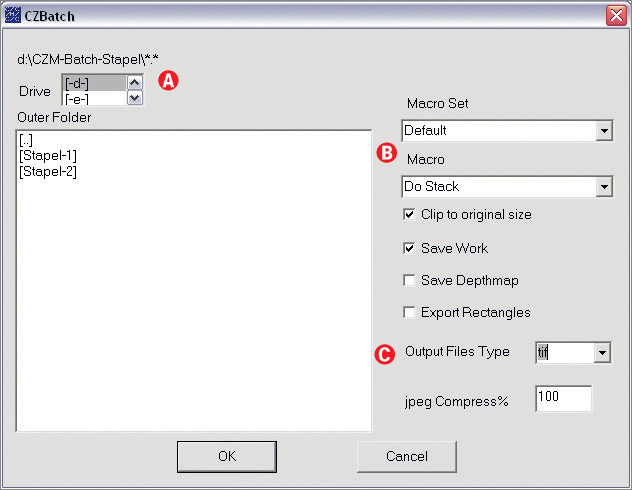
Figure 4-38: CZBatch allows you to batch process multiple stacks. The merged images are saved in a folder called “CZMOutputs”. The illustrated dialog box allows you to select which macro is to be used for processing, and which format your merged images will be saved to.

In the CZBatch program window (see figure 4-38), you can select the folder containing your sub-folders (stacks), select the macro you wish to apply, and select your desired export format.

CZBatch then runs through the individual folders, processing the images therein by passing the individual steps to CombineZM via a command prompt. The resulting merged images are exported to a folder called CZMOutputs, and are given the same name as the folder containing the source frames for the merge stack.

The online discussions conducted in various forums indicate that CombineZM is often used to merge multiple photomicrographs (shot using a microscope), with the aim of enhancing depth of field for this medium too.

Photomicrographic images often have a very shallow depth of field, and enhancing their depth of field can help to make them easier to interpret. The source images for such sequences are often taken using inexpensive webcams with sensor resolutions as low as 1.3 megapixels, and attached to the microscope using home-made adapters. Such low resolutions are not usually a problem when shooting photos through a microscope.

Given the large numbers of shots such procedures require, it is useful to control focus for the individual shots using a computer-controlled stepper motor. There are, these days, a number of macros available online written exactly for this purpose.

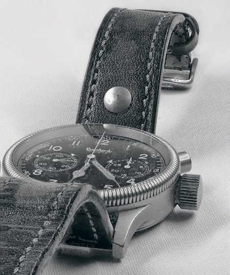
Figure 4-39: This image was also created from eight source images that were merged using CombineZM.

4.7 Focus Stacking Using Helicon Focus

Our attempts at focus stacking using PhotoAcute worked smoothly, but didn’t always produce optimum results. The focus stacked images we produced using CombineZM ranged from excellent to unacceptable. The surprising thing was that we managed to produce varied (and sometimes non-reproducible) results, even using exactly the same source images and program settings. This is why we decided to also test Helicon Focus (from HeliconSoft [17]), although this wasn’t part of our original plan.

Helicon Focus is available for both Windows and Mac OS X, and can be used for stitching processes as well as the focus stacking functionality we will describe here. The program is available in both Lite and Pro versions. The Pro version has additional functionality, including a retouching brush which you can use to transfer whole portions of the scaled and aligned source image directly into the target image. The Windows version of the program also includes a batch processor, and allows you to export animated stacks. Both professional versions include a panorama function and support multiple processors, which can help increase your processing speed if you are working with large stacks or stacks containing large image files.

The Mac version is only available with an English language interface, while the Windows version (which we will describe later) has a multi-language interface, including German, French, and Spanish.

Helicon Focus can be bought with a limited, one-year license or an unlimited license, which is approximately 3½ times more expensive. An unlimited license includes free access to all future updates to the program.

We recommend starting with the free 30-day trial version. If you decide you want to continue using the program, you can then purchase the Lite version, which you can always upgrade later if you need the additional functionality offered by the Pro version.

A useful Helicon Focus support forum can be found at: http://forum.helicon.com.ua/

Of the three programs PhotoAcute, CombineZM, and Helicon Focus, Helicon Focus has the best, most user-friendly user interface, making the program intuitive and easy to use.

You will need to set your basic preferences when you start the program for the first time. We used the settings illustrated in figure 4-40. We discovered that the Mac version took a very long time to find the folder containing our image editor (in our case, Photoshop CS3), but this setting only has to be made once, and was thus not a serious problem.

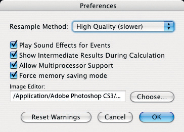
Figure 4-40: You need to set your basic preferences when you start the program for the first time.

For our stacking example, we used the four images of a withered tulip which can be seen in figure 4-41 to produce a single, final image with maximized depth of field. The source images were shot in daylight using a 10-megapixel Nikon D200 and a Nikkor 60 mm f/2.8 macro lens set to f/9. We used manual focus and shot from a tripod.

Once again, the first step is to load the source images into the program using File ▸ Add Image, or by clicking on the Open icon and navigating to the directory that contains the source files.

Figure 4-41: Our source images of a withering tulip, shot using four different focus settings.

Alternatively, Mac users can also drag and drop their source files from an image browser (such as Adobe Bridge, or the Mac OS X Finder). Dragging and dropping only works in the Mac version. In Windows you have to use the Open dialog to load your source images.

Once the images have been loaded, the program displays the currently selected image in a central preview window (see figure 4-42).

You can review the individual images using the Source Files list at the top left of the preview window. You can zoom in to each image using the keystroke, or by clicking the zoom-in button . Clicking or using zooms back out. In Windows, the fastest way to zoom is using the size slider located beside the icon.

Use the Rotate Right or Rotate Left button to rotate your images if needed.

As in our previous examples, you should make sure your images are loaded in the order they were shot and/or focused. And remember, only images with a checkmark will be processed.

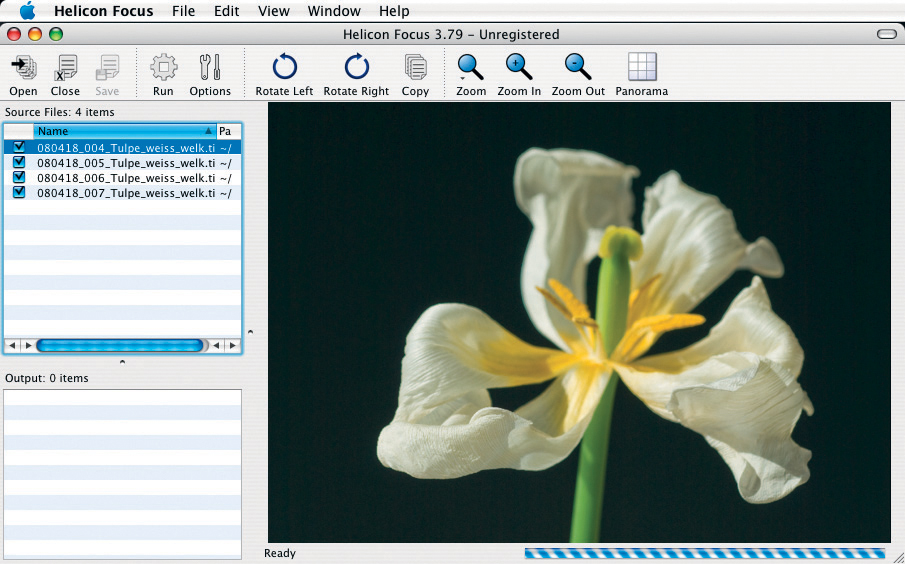
Figure 4-42: The Helicon Focus program window. The four source images are already loaded and activated (checked), and the program is displaying the first image in the preview window.

You can use the Options () button to set a number of other processing preferences (see figure 4-46 on page 83 and figure 4-47 on page 84). For a first attempt, the default settings should be fine.

A single click on Run , or using the keystroke will start the Helicon Focus stacking operation. During the process, the progress bar at the bottom of the main window will help you to estimate the remaining processing time. Our quad-processor Mac and Helicon Focus Pro processed the job fairly quickly, in spite of the fact that we were using relatively large 16-bit TIFF files.

Once merged, the final image will appear in the program’s output list and will be displayed in the preview window (see figure 4-43).

The resulting image (created using the standard settings illustrated in figures 4-46 and 4-47) is not as sharp as those created using PhotoAcute or CombineZM – but is by no means out of focus.

This fits into our personal workflow very well, as we prefer to sharpen our images later using Photoshop (using the USM filter, for example), and to a degree that is suitable for our chosen output medium. This helps us to avoid over-sharpening, and to apply selective sharpening effectively only where it is really necessary. We perform this final sharpening using a layer mask, as described in section 7.2.

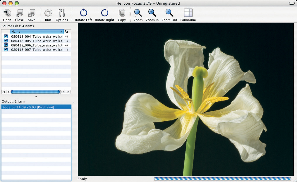
Figure 4-43: The stacked image with its extended depth of field appears automatically in the program’s output list.

If you want to increase sharpness from the outset, you can reduce the strength of the Smoothing parameter (found in the General tab of the Options dialog; see figure 4-46).

The final step is to save the image using File ▸ Save Image. Here too, you can select various output formats. If you are planning to do retouching using Photoshop, we recommend using the 16-bit TIFF format, as the lossless LZW compression algorithm used for TIFF images gives you the most leeway for applying selective sharpening or increasing local contrast later. Your input format will always determine your output format as far as this is possible – the TIFF and PSD formats support 16-bit input and output, for example, whereas JPEG can only be saved at up to 8-bit color depth. The Helicon Focus export formats include JPEG, JPEG 2000, PNG, TIFF and PSD (see figure 4-44).

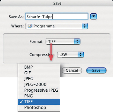
Figure 4-44: Helicon Focus offers a number of different output formats for your merged images.

Figure 4-45 shows our final image after it has been post-processed using the DOP Detail Extractor filter described in section 7.1. The extractor has helped to increase the image’s microcontrast so that the delicate structures of the flower’s petals stands out more. The image has also been slightly cropped.

Helicon Focus offers a number of options when processing focus stacks, which can be found under Options (or by clicking on ).

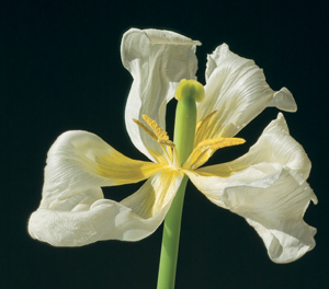
Figure 4-45: The result of the Helicon Focus stacking process. We improved microcontrast and applied some slight sharpening at the post-processing stage.

One of the most important Options parameters is the Radius setting (see figure 4-46). This determines the size of the pixel radius that will be used to determine which parts of the source images are in focus, and will therefore be used in the final, merged image. The second important parameter is Smoothing, which controls the overlay mechanism function that merges the separate parts of the various source images. A low smoothing value leads to sharper images, but can cause some image artifacts to appear. A higher smoothing value results in smoother (but softer) transitions from image area to image area. The Image Processing method selection menu is only available in the Pro version of the program and currently contains two options, A and B. In our tulip example, the differences between the results produced by the two methods were virtually undetectable. For the stacked shot of our old Leica (see the illustration on page 73), Method B produced slightly better results with less visible artifacts.

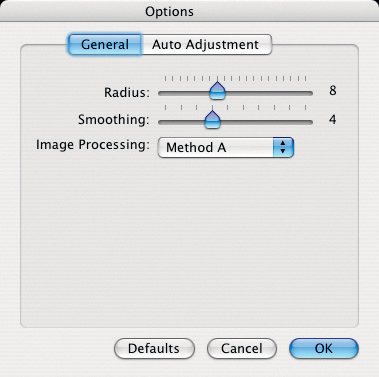
Figure 4-46: Two important settings in the Helicon Focus “Options” dialog.

The settings found on the Auto Adjustment tab (see figure 4-47) control how your images are prepared for the focus stacking process. These include how the source images should be aligned, to what degree they can be realigned, and the maximum allowable angle of rotation. The Magnification value specifies a percentage to which each image can be scaled, should this be necessary in order to achieve the required focus effects. The final parameter relevant to focus stacking is Brightness, which controls the degree to which Helicon Focus matches source image brightness, if at all.

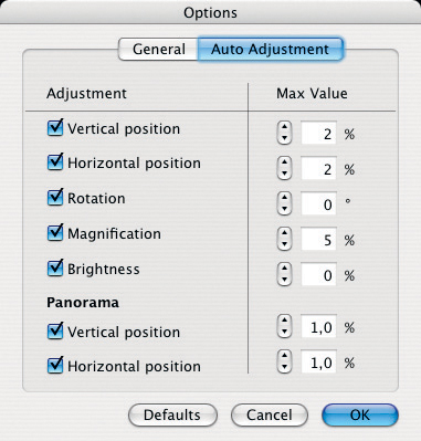
Figure 4-47: The parameters provided in the “Auto Adjustment” tab allow you to specify how the alignment of the source images should be done.

If you work with a tripod, the default parameters usually produce acceptable results. However, if you are shooting hand-held (never a good idea for macro shots), then it may be necessary to increase the values of the first four parameters.

Dust Maps

Helicon Focus also offers the special Dust Map function, which allows you to map the positions of any dead or hot pixels, or dust particles which may have been present on the image sensor during shooting. These erroneous pixels are then ignored by the program during processing and the resulting gaps are instead interpolated from neighboring pixels.

To use the function, you need to create a separate empty, white frame at the start or end of your sequence. Helicon Focus then uses this image to create the dust map. The frame should be shot against a white surface, out of focus, and at exactly the same size as your other source images (if you preprocess or convert your images before processing).

The dust map is loaded at the end of your sequence using File ▸ Add dust map. You can then start processing in the normal way.

Opacity Maps

Despite its generally effective functionality, Helicon Focus sometimes fails to merge a sequence correctly. This could be caused by several images having the same image area in focus, making the program incapable of deciding which image to take these pixels from. In such cases, you can have the program generate Opacity Maps for later use in Photoshop. You can also simply remove an image that might be causing problems from the input sequence and try again.

Helicon Focus for Windows

Helicon Focus for Windows is more highly developed than its Mac counterpart. This is evident from the version numbers (the latest Mac version is 3.79, while the Windows version is already at 4.60). Handling of both versions is very similar, except for the fact that the Windows version is capable of processing Canon RAW files. Figure 4-49 shows the main user interface for the Windows version of the program.

To start the process, load your source files into the program using the function. As usual, multiple images can be selected by holding down the key, or use to select non-adjacent files from the browser window.

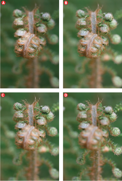
Figure 4-48: Our four source images of a fern were taken using a Canon 100 mm f/2.8 macro lens, and using the built-in flash on a Canon 40D. The images were shot from the (minimum) distance of 12.5 inches at f/11.

If you are working with RAW files, you should expect the loading process to take longer than it would take for JPEG or TIFF files. We have found that Helicon Focus’ RAW processing capability is not particularly powerful, so we recommend that you convert your RAW files to 16-bit TIFF before processing them using this program.

You can use the program’s window icons to change the appearance of the user interface. You can choose between a single window (), two horizontal halves (), or two vertical halves (). Working with a split screen allows you to view the source images and the merged image simultaneously.

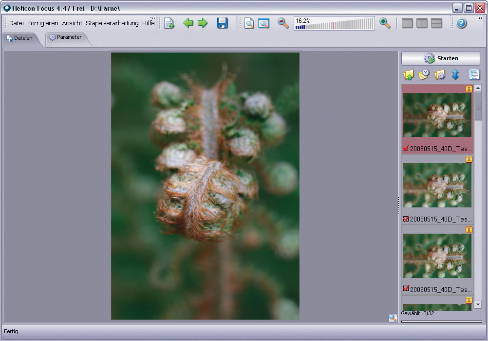
Figure 4-49: The Windows version of the Helicon Focus main window, showing the list of loaded and activated source images.

Next, you can view your source images. If an image has been loaded in RAW format, it will only appear as a preview once you click on its listing.

Pressing will rotate an image 90° to the right, and will rotate it 90° to the left, although it is preferable to rotate your images before loading them. Clicking on the zoom scale allows you to quickly enlarge and reduce the preview image, and moving the mouse over the image causes a magnifier to appear, helping you to examine image detail. Clicking the icon displays a histogram and some of the EXIF data associated with the currently selected image.

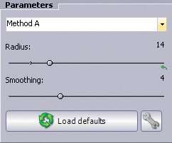
Figure 4-50: The “Parameters” tab includes the three most important merge settings.

We now check and set the processing parameters located in the Parameters tab (see figure 4-50) previously described on page 83. General preferences can be set by clicking on View ▸ Preferences (see figure 4-51). The palette will display four tabs: General, Autoadjustment, RAW, and Cache. We recommend deactivating option under General (see figure 4-51), because it speeds up processing. If you do not have much RAM available, it is also a good idea to activate option .

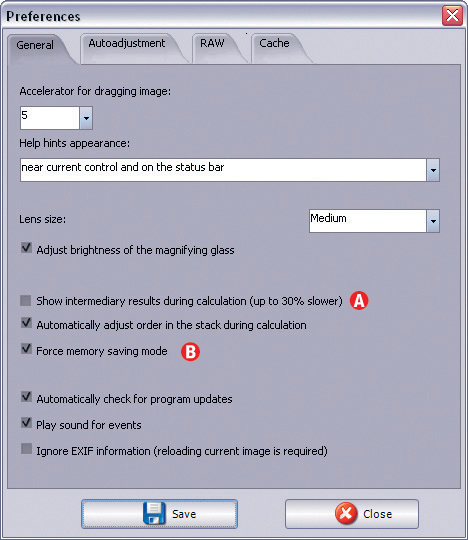
Figure 4-51: These general preferences can be found under View ▸ Preferences. We recommend using the program’s default presets.

In the Automatic Correction tab (see figure 4-52) you will find the correction parameters described on pages 83 and 84. Here is a quick summary:

The settings Horizontal position, Vertical position, Rotation and Magnification determine to what degree the individual images in the stack can be shifted, rotated, or scaled in order to achieve optimum image overlap.

The default values are well chosen, but you may need to raise them slightly if you are processing shots that were taken hand-held or in wind. Any increases will lengthen the time it takes to process the images. If you changed the lighting conditions while shooting, it is best to increase the Brightness value from 0 to about 5% or 8%. The two additional parameters are only relevant to micro-panorama sequences.

The settings listed in the RAW tab (see figure 4-53) allow you to determine how RAW files will be processed. One possible variant is to have Helicon Focus use the well-known dcraw converter, which is free, but doesn’t quite produce the same quality of image that commercial programs such as Adobe Camera Raw, Lightroom, Apple Aperture, or Capture One can achieve.

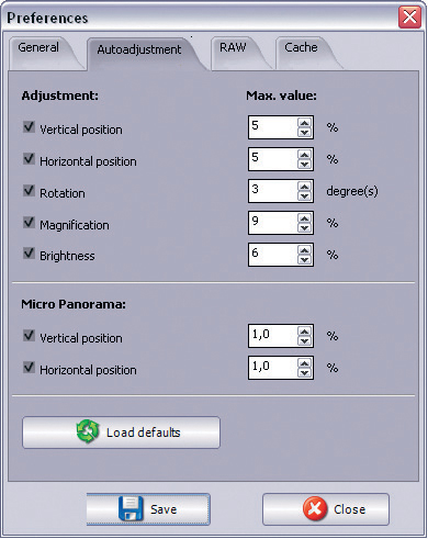
Figure 4-52: The image alignment settings.

Whether you choose to activate dcraw, and which manufacturer’s RAW format you are processing, dictates which options can be adjusted. The meaning of the varies options on offer requires some foreknowledge of the working of RAW converters. This is another good reason to work with 16-bit TIFF files or 8-bit JPEG files while using Helicon Focus.

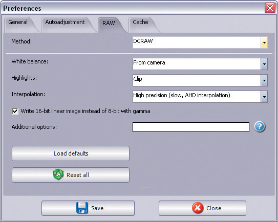
Figure 4-53: The RAW tab includes the settings for processing RAW images. The available options vary depending on which RAW format you are using.

You can use the Cache tab to set the location of the program’s cache files – we recommend using a disk with plenty of free space and fast read/write speeds. It is a good idea to periodically empty both cache locations, as these can quickly fill up with buffer data and preview thumbnails.

Don’t forget to save the changes you make to the program settings by clicking the Save button . Changes made in any of theses tabs are only activated once they have been saved and the program has been restarted.

We can now begin the actual processing by clicking the Start button . Only selected images (indicated by a red check mark) will be included in the focus stacking process.

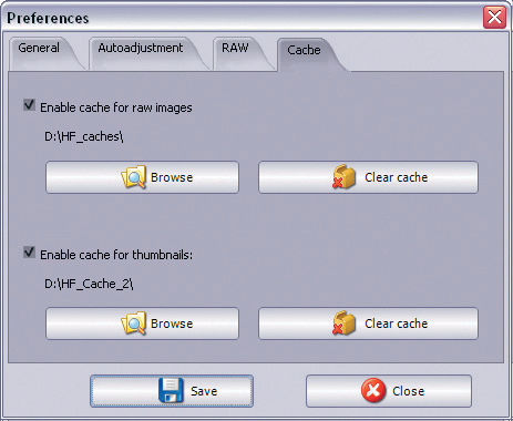
Figure 4-54: The “Cache” tab allows you to define where Helicon Focus will save its cache files.

If your initial results are not as good as you had hoped, the first thing to change is the Method. In our example, Method B worked better than Method A. If this still doesn’t help, you can also adjust the Radius and Smoothing parameters. If you are still not satisfied, you will have to make changes to the program’s basic preference settings. Unfortunately, the Windows version of Helicon Focus cannot save individual preference configurations for later use.

Figure 4-57 on page 90 shows the first resulting image processed using the default parameters and Method B. The image has good depth of field in the foreground, but the merging process for the unsharp background has not really produced satisfactory results. The original was actually better (see figure 4-48 on page 85).

To remedy this, we copied some of the soft-focus areas from the first image in our stack to the merged image using a large, soft retouching brush tool. This tool is currently only available in the Windows version of Helicon Focus and is located in the Retouching tab (see figure 4-55).

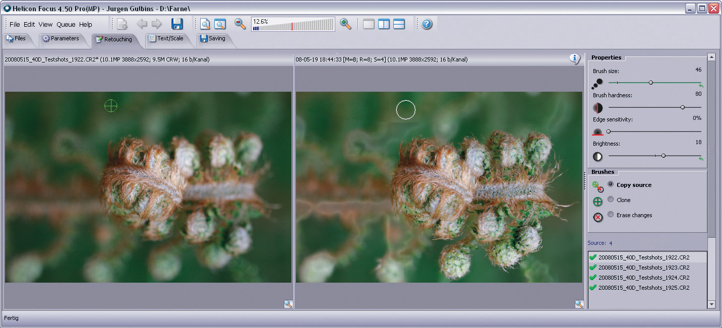
Figure 4-55: The editor found in the “Retouching” tab allows you to copy elements from your source files into the merged image.

The brightness of the merged image was automatically adjusted by the program. Therefore, we set the Brightness slider to 5%, making it necessary to match the brightness of the source image with that of the merged image when copying. This is achieved using the Brightness slider shown in figure 4-55.

We could also have carried out this correction using the Photoshop Clone Stamp tool , but the images in Helicon Focus are already rotated and scaled, and the program supports the matching of image brightness. Figure 4-58 shows the final image, generated and corrected exclusively using Helicon Focus.

Clicking on the icon will then initialize the Save dialog. Because we almost always perform our post-processing using Photoshop (described in sections 7.1 and 7.2), we choose either TIFF (compressed using the LZW algorithm), or Photoshop’s native PSD format. Helicon Focus automatically includes the Method, Radius, and Smoothing parameters in its file names, which can be helpful while you are learning to use the program. If your input files are 16-bit data, your output file will also be 16-bit data.

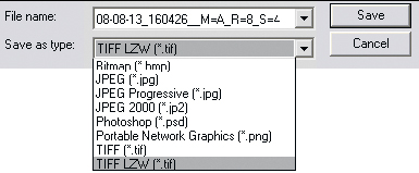
Figure 4-56: The Windows version offers more output formats than the Mac version.

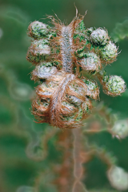
Figure 4-57: Our initial merged image, created from the source images shown in figure 4-48.

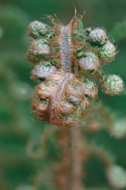
Figure 4-58: Our image after editing using the Helicon Focus retouching tools. The artifacts visible in figure 4-57 are almost gone.

Clicking on the Save tab displays the options shown in figure 4-59. The Create animation option allows you to save a film showing the actual merging process taking place, which can be viewed in a web browser.

The Windows version of Helicon Focus transfers the EXIF and IPTC data from the first image in a stack to the merged image. This feature is not available in the 3.79 version for Mac.

The automatic transfer of IPTC data does not work with RAW files. This is because no currently available image management program is capable of writing this data directly into the image file. These data are usually either saved separately in the image database, or, in Adobe’s case, in an XMP “sidecar” file. Most third-party programs (including Helicon Focus) cannot access this data.

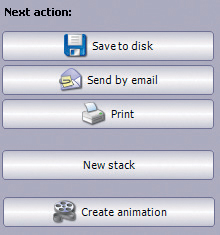
Figure 4-59: The “Save” tab offers options for printing, mailing, or animating your results.

Batch Processing

Instead of immediately processing a stack of selected images using the current settings by clicking Start, you can also use Add to the queue (at the bottom right of the Parameters tab) to queue the stack for batch processing.

Pressing will display the batch queue (see figure 4-60) along with a choice of export formats and save locations. Here, you can also delete individual entries from the current queue.

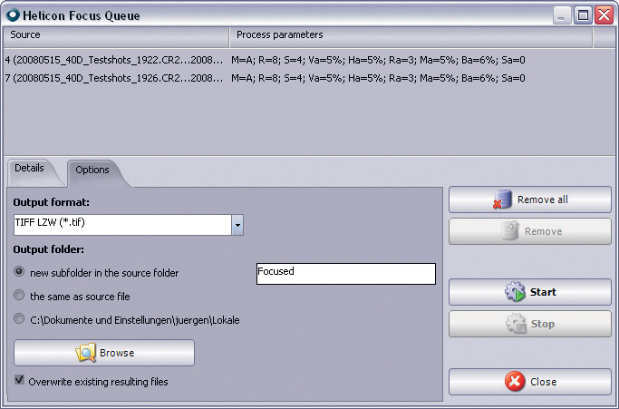
Figure 4-60: Pressing displays the Helicon Focus batch processing queue.

Clicking the Start button causes the queued stacks to be processed one after another, while you take a well-earned coffee break. Performing other tasks on your computer while Helicon Focus is batch processing can be difficult, as the program will use most of the computer’s available memory and processor power for the job.

4.8 Semi-Automatic Focus Stacking Using Photoshop CS4

We had the opportunity to try out Photoshop CS4 shortly before this book went to press, so we are including a section describing the new CS4 functionality here.

As described in section 4.4, the first step is to load your source images into separate layers and align them. This is done using File ▸ Scripts ▸ Load Files into Stack. If you archive your images using Adobe Lightroom, it is easier to use Photo ▸ Edit in ▸ Open as Layers in Photoshop. In the dialog that follows, activate the Attempt to Automatically Align Source Images option (see figure 4-8 on page 62).

This time, we will use the three source images of a withered iris shown in figure 4-61. Each of the three shots shows very different lighting conditions, making the entire process more difficult.

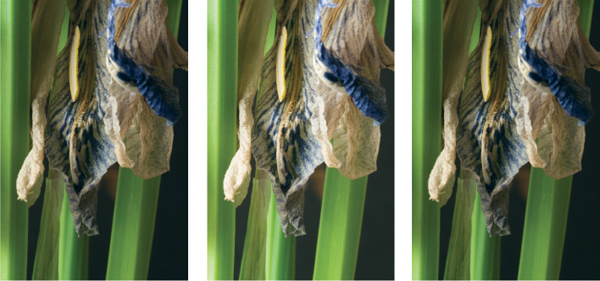
Figure 4-61: Three shots of a withered iris used as source files for a semi-automatic focus stacking run in Adobe Photoshop CS4.

We now crop our images so that only detail-rich areas remain. Our layer palette now looks like the one illustrated in figure 4-62.

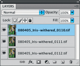
Figure 4-62: The Layers palette with our aligned images on three layers.

Next, we select all layers (not only the top layer) and use Edit ▸ Auto-Blend Layers. Photoshop will display a dialog (see figure 4-63) in which we select the type of blending we wish to use. In this case, we select Stack Images. We also activated the Seamless Tones and Colors option.

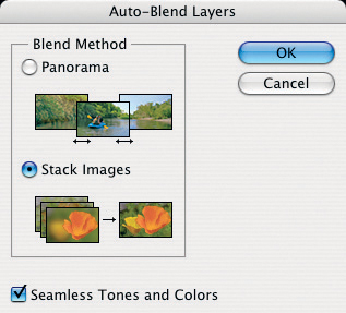
Figure 4-63: Select your desired blending method.

Clicking OK starts the blending process, which is actually quite fast in Photoshop. Figure 4-64 illustrates the layer masks thus created – the images are still there in their own layers and not yet merged to a single layer. This can be quite useful, as it allows you to fine-tune your image by further refining the individual masks.

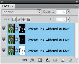
Figure 4-64: The Layers palette after the blending process has finished.

Our Photoshop CS4 results were not quite as good as those produced by Helicon Focus. The merged (blended) image shown in figure 4-65 still shows a number of artifacts (the white leaf at the left, for example, still shows some ghosting), and it is obvious we should have shot additional photos covering the very front of the scene. This type of blending functionality is still in its infancy in Photoshop, but it is nevertheless well worth trying for some scenes.

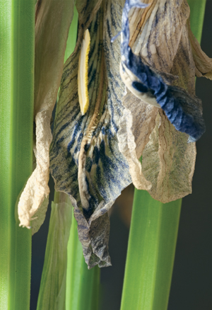
Figure 4-65: The result of the blending operation done using Photoshop CS4 merging the images of figure 4-61. The result is definitely not perfect, as a number of artifacts indicate, but some retouching using the Photoshop clone tool and by editing the layers masks could fix this.

While Photoshop CS4 might not currently be the best available application for focus stacking, its loading and image alignment functionality is quite good.^* These features can be used to prepare images for HDRI merges using other programs, such as FDRTools, or even Photomatix Pro. You can export aligned and cropped image layers to separate files by selecting the appropriate layers and using File ▸ Scripts ▸ Export layers to Files.

4.9 Focus Stacking – A Summary

For focus stacking processes, Helicon Focus was our favorite program. It is fast, very reliable, offers more options than PhotoAcute, and unlike CombineZM, it can process 16-bit images and RAW files. Of these three specialized programs, it also offers the most comprehensive online manual.

The only real disadvantage is its price. For users who do a lot of work shooting for focus stacking – possibly even professionally – the investment will soon pay for itself. Also, working with Helicon Focus is fun.

In our test version (Mac Version 3.79) we missed the ability to save entire settings profiles for later re-use. The Helicon Focus forum is abuzz with talk of the upcoming version five, so we can expect to see this function incorporated into the program soon.

Just as with PhotoAcute and CombineZM, the 3.79 Mac version of Helicon Focus cannot incorporate EXIF or IPTC data from source files into the processed image. The Windows version has this capability.

You can enter IPTC data for processed images by hand, but special programs are required to do the same with EXIF data.^* We recommend using the Exactor freeware by Phil Harvey [41], which also lets you copy IPTC, EXIF, GPS, and/or XMP data. ExifTool is available for both Windows and Mac OS X. Another option is the shareware program EXIFutils [47]. This is actually a whole suite of command-line-based tools which run on Windows, Mac OS X, and Linux. The freeware program Exifer [45] is also quite effective, but is only available for Windows.

In the current 4.60 Windows version of Helicon Focus, the program extracts EXIF and ITPC data directly from the first image of a stack and applies them to the merged image. This is a great feature, and we expect it to be included in the Mac version of the program soon.

If you only want to process a few straightforward images, Photoshop can be used to produce acceptable results quite quickly using layers masks. However, if you are dealing with large numbers of images (such as large stacks of images shot through a microscope), automated processes are faster and more reliable. We also generally recommend PhotoAcute, although it offers less flexibility than Helicon Focus. CombineZM reaches its limits quite quickly when confronted with large image files, and doesn’t support 16-bit processing. The CombineZM internet forum, however, indicates that the program enjoys widespread use, and it does, of course have the distinct advantage of being free.

All three of these specialized programs are constantly undergoing further development, so it makes sense to check for updates and improved versions on a regular basis.^** You will often find that bugs and open issues from earlier versions have been fixed in the latest downloads.

Focus stacking is still a highly specialized niche in the photographic world, but can make obvious improvements to certain types of scenes. In the field of photomicrography, the technique is virtually a necessity.

Figure 4-67 shows an image created by merging the source photos shown (reduced) in figure 4-66. We created the merged image using Helicon Focus set to Method A, a Radius of 5, and the Smoothing value set to 2.

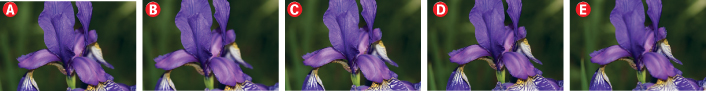
Figure 4-66: Five photos of an iris taken using a macro lens. This sequence portrays the different sharpness layers moving from front to rear of the scene.

Our first result contained some unsightly background artifacts, which we removed using Photoshop. We achieved this by loading the source image (figure 4-66 ) and the composite image on top of each other. We then used the Clone tool to copy the out of focus (but smooth) background of the first image into our final image. We also removed some slight color fringing artifacts from around several of the leaves in the foreground using the Clone tool.

Once you have tried focus stacking technology, we are sure you will want to use it time and again.

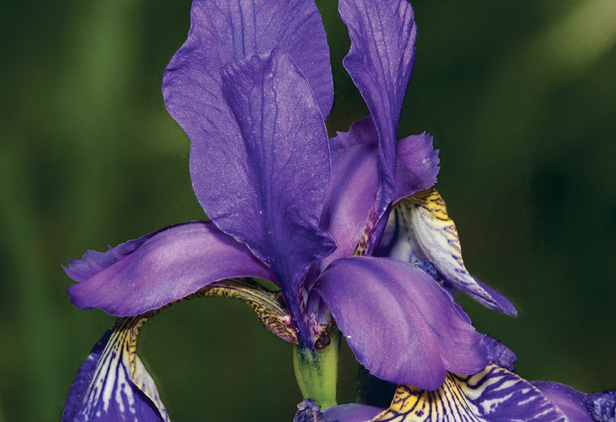
Figure 4-67: This image was created by merging five source files (see figure 4-66) using Helicon Focus. Some artifacts that appeared at some of the leaf edges were eliminated using Photoshop’s clone tool.