11 Data Fragmentation

In a distributed database system, two major questions are (1) how the entire set of data items in the database can be split into subsets and (2) how the subsets can be distributed among the database servers in the network. Question (1) addresses the problem of data fragmentation (also called sharding or partitioning); Question (2) addresses the problem of data allocation.

We first survey properties and types of fragmentations from a theoretical point of view and then discuss fragmentation approaches for different data types.

11.1 Properties and Types of Fragmentation

What good fragmentations and good allocations are for a given database highly depends on the runtime characteristics of the system. In this sense, the query behavior of users plays an important role for the quality of fragmentation and allocation: for example, properties to be considered for the fragmentation and later on allocation of the fragments could be:

–the type of accesses (mostly reads or mostly writes),

–the access patterns (which data records are accessed regularly and which only rarely),

–the affinity of records (which data records are accessed in conjunction with which other data records),

–the frequency of accesses and

–the duration of accesses.

Once a good fragmentation and allocation have been established, a distributed database can take advantage of

–data locality (ideally, data records in the same fragment are often accessed together),

–minimization of communication costs (ideally, no data records have to be moved to another server in order to answer a query),

–improved efficiency of data management (ideally, queries on smaller fragments can be executed faster than on the large data set and index structures can be smaller and hence data records can be found faster),

–and load balancing (ideally, all servers get assigned the optimal amount of data and only have to process user queries according to the capacities of each server and without the danger of hotspots – that is, without overloading a few servers with the majority of user queries while the other servers are mostly idle).

However, a given data distribution is in general not optimal for any kind of queries that a user may come up with. Hence, on average a fragmented database system has to live with several disadvantages. In particular, queries that involve subqueries over different fragments are costly because the global query has to be split into subqueries (a process called query decomposition), the affected fragments have to be identified (a process called data localization) and data records have to be sent over the network to computed the final result. Moreover, distributed transactions are extremely difficult to manage: in case of concurrent accesses, system-wide consistency can be maintained only with very complex processes; the same applies to distributed recovery when one or more servers crashed during such a transaction.

Several criteria are important when designing a distributed database with fragmented data sets and when developing algorithms for the maintenance of data fragmentation. The first and foremost demand is that a given data fragmentation must be correct in the sense that the original data set can be entirely reconstructed from its fragmented representation. When the data set is recombined from the fragments, the following two correctness properties are required:

Completeness: none of the original data records is lost during fragmentation and hence no data is missing in the reconstructed data set; in other words, completeness means that each bit of data from the original data set can be found in at least one of the fragments.

Soundness: no additional data are introduced in the reconstructed data set; in other words, only data that belong to the original data set can be reconstructed.

More formally, for a data set D, let D₁, … , D_n be its fragments. Let ⊙ be an operator that combines the fragments (for example union or join). Correctness of the fragmentation then ensures that D = D₁ ⊙ … ⊙ D_n.

Additionally, non-redundancy can be fulfilled as an optimality criterion: any fragment should be minimal in the sense that it does not overlap with any other fragment. More formally, for any two fragments D_i and D_j (where i ≠ j), it ideally holds that D_i∩D_j = . However, as we will see shortly, some redundant information might be necessary to allow for reconstruction (for example, by using tuple IDs or shadow nodes).

In order to be practical for large data sets that are frequently modified, many more requirements are necessary for an efficient long-term management of the distributed data sets (some of these properties are also summarized in [AN10]):

Unit of distribution: the individual data records that the fragments of the data set are composed of should neither be too coarse nor too fine-grained. If data records are too coarse (like entire relational database tables), the fragmentation becomes inflexible. If data records are too fine-grained (like individual attributes inside an object or inside a vertex) logically coherent entities are split and their data is separated into different fragments: this would soon make the fragmentation (and later on the query processing) inefficient.

Fragment sizes: The sizes of the obtained fragments should be configurable in the fragmentation algorithm. This facilitates load balancing in the distributed database system. In particular, equally sized fragments are advantageous for an efficient load balancing in a network of homogeneous server.

Workload awareness: Some fragmentation approaches consider only the data records stored in the database system, while others estimate what a typical sequence of read and write requests (a so-called workload) in the distributed system will be; and then they optimize the fragmentation with respect to this workload. One aim of a workload-aware fragmentation will be to optimize efficiency of distributed query processing. This means on the one hand, that queries should be answered within a single fragment and without crossing fragment boundaries. This is particularly important when the recombination of the fragments is costly – like a distributed join or navigational access in an XML tree or a graph; it is less a problem where subquery results are recombined by just taking their union – like in key-based access in key-value stores or extensible record stores. On the other hand, workload-aware fragmentation should avoid hotspots where most of the queries will affect only a small set of the fragments; instead, queries should be distributed well among all fragments. Workload-aware fragmentation can hence lead to a balanced distribution; but it is more complex than data-dependent fragmentation, such that it might be inappropriate for a distributed database system with real-time constraints.

Local view: The local view property of a fragmentation algorithm means that fragments can be computed by just looking at a small part of the data and processing the data set step by step. That is, there is no need to have information about the entire data set (or even load the entire data set into memory); fragmentation algorithms that need a global view of the entire data set are usually impractical for a distributed database system.

Dynamic adaptation: An existing fragmentation can be adapted upon modifications in the data set. An algorithm can be run on the existing fragmentation (possibly in several iterations) to improve it and adapt it to the new situation. Distributed computation: The process of fragmentation can be distributed among different servers. In particular, for an existing fragmentation, each fragment can be modified by the server it is assigned to.

Apart from these desired properties, fragmentations can be achieved in different ways. Types of fragmentation algorithms include:

Handmade: A handmade fragmentation requires a database administrator to identify fragments in a data set and set up the database system accordingly. Fragmentation by hand is only feasible on a very high abstraction level. For example placing employees of a company into a fragment for their department in the company node, works on the abstraction level of the department. A more fine-grained abstraction level quickly becomes infeasible to maintain by hand. For example, configuring fragments for working groups of employees where often new working groups are created or employees switch their groups will be difficult to set up and keep track of.

Random: In a randomized fragmentation, every data record has the same probability to be assigned to a fragment. This is a simple procedure that satisfies many of the above properties like local view and supporting dynamic additions of data records. Keeping partitions equally-sized requires some more complex probability distribution if data records can be deleted and thus some fragments shrink quicker than others. On the downside, random fragmentation is not workload-aware with the effect that the randomized process may cause excessive communication load between fragments or may create hotspots.

Structure-based: A structure-based fragmentation looks at the data schema definition (or the data model in general) and identifies substructures that constitute the fragments.

Value-based: A value-based fragmentation looks at the values contained in the data items to define the fragments. For example, by specifying some selection predicates the values contained in some fragments can be constrained. Several such selection predicates can be combined into so-called minterms [ÖV11]: the minterms correspond to disjunctions of selections so that each minterm defines one fragment that is disjoint from the other fragments. The structure (and hence if available the schema of the data) is not altered.

Range-based: As a special form of value-based fragmentation, range-based fragmentation splits the primary key (or another attribute that can be sorted) into disjoint but consecutive intervals. Each interval defines a fragment.

Hash-based: If each data record has a key (for example, the key of a key-value pair) the hash of this key can determine the database server that the data record is assigned to. In this setting, each database server in the distributed database system is responsible for a subrange of all hash values.

Cost-based: Cost-based fragmentation relies on a cost function for finding a good fragmentation. The aim is then to find a fragmentation with minimal overall cost. For example, for a graph data model a typical cost function is the number of crossfragment edges where one node of the edge lies in a different fragment than the other node; the number of such inter-fragment edges – the so-called edge cut – should then be minimal to reduce communication costs when traversing edges. For a more realistic cost estimation, workload awareness can then be added to the cost-based fragmentation process: for a given sample workload the aim is to find a fragmentation that minimizes the cost of the given workload. For the different data models different cost functions may be used. For example, in the case of the graph data model we might for example only minimize the edge cut for edges that are traversed in the sample workload whereas other (non-traversed) edges can be ignored.

Affinity-based: This form of fragmentation is based on a specification of how affine certain data records are – in other words, how often they are accessed together in one read request.

Clustering: Specialized algorithms can be used for finding coherent subsets in the data (so-called clusters). Clustering algorithms often apply heuristics that do not find a global optimum but find a near-optimum solution quickly.

11.2 Fragmentation Approaches

Depending on the data model chosen, different ways of fragmenting data are possible and require different recombination methods. This sections surveys some of them.

11.2.1 Fragmentation for Relational Tables

In relational database theory, several alternatives of splitting tables into fragments have been discussed (see for example [ÖV11]). The two basic approaches are vertical fragmentation and horizontal fragmentation. In addition, derived fragmentation is based on a given horizontal fragmentation and hybrid fragmentation combines both vertical and horizontal fragmentation:

–Vertical fragmentation: Subsets of attributes (that is, columns) form the fragments. Hence, vertical fragmentation is a form of structure-based fragmentation. Rows of the fragments that correspond to each other have to be linked by a tuple identifier. That is, a vertical fragmentation corresponds to projection operations on the table such that all fragments have a different database schema (with only a subset of the attributes). The fragmented tuples can then be recombined by a join of all fragments over the tuple identifier. To illustrate this consider the original data in Table 11.1 that is split into two fragments with an additional tuple identifier (ID). This is an example for an affinity-based vertical where columns A, B and C, D are assumed to be more affine than other subsets of columns (that is, they occur in the same transaction very often for a given workload). For different workloads, affinity may change; for example, if columns B and C are more affine than columns A and B, then columns B and C might be placed in one fragment while columns A and D together form the second fragment.

–Horizontal fragmentation: Subsets of tuples (that is, rows) form the fragments. A horizontal fragmentation can be expressed by a selection condition on the table with the effect that all fragments have the same database schema (which is identical to the original database schema). Hence, horizontal fragmentation is a form of value-based fragmentation. Recombination is achieved by taking the union of the tuples in the different fragments. In the example in Table 11.2, the first two rows form the first fragment while the last row constitutes the second fragment.

–Derived fragmentation: A given horizontal fragmentation on a primary table (the primary fragmentation) induces a horizontal fragmentation of another table based on the semijoin with the primary table. In this case, the primary and derived fragments with matching values for the join attributes can be stored on the same server; this improves efficiency of a join on the primary and the derived fragments.

–Hybrid fragmentation: A hybrid fragmentation denotes an arbitrary combination of horizontal and vertical fragmentation steps. The more fragmentation steps are combined, the more complex it is to recombine the original data set. The fragments then differ much in the schemas that they have to follow.

11.2.2 XML Fragmentation

A recent comprehensive survey on XML fragmentation is given in [BM14]. For XML fragmentation the first distinguishing feature is whether a set (a “collection”) of XML documents must be fragmented into subcollections or a single large XML document must be fragmented into subdocuments. In the first case (fragmentation of collections), a large collection (of small XML documents) is divided into subcollections which can each be stored on different servers.

–A value-based (sometimes called horizontal) fragmentation of a collection is defined by selection operations on the XML documents that identify the subcollections. For example, in a collection of XML documents describing departments of a company, the European departments can form one subcollection (for example by selection on a location element with value ‘Europe’) while the American departments form another (by selection on a location element with value ‘America’). If the documents in the original collection obeyed an XML schema definition then the documents in each of the subcollections also obey the same schema.

–A structure-based (sometimes called vertical) fragmentation of a collection splits the XML schema definition of the original collection into separate schema definitions that all specify subtrees of the original documents. Hence the structure-based fragmentation of the collection leads to a fragmentation of each document contained in the collection. Continuing the above example, all subtrees of all documents describing the location of each department will be stored in one collection, while all subtrees describing the staff will be stored in another collection and hence both subcollections have their own schema.

A single large XML document can also be fragmented: it is split into subtrees. Fragmentation of such a document can be divided into value-based fragmentation and structure-based fragmentation, too. In a value-based fragmentation, the large document is split into subtrees by applying selections to it based on values stored in text nodes. Similar to the example above, when a document contains information on all departments of a company, value-based fragmentation can extract one subtree for all European departments (where a location element has the value ‘Europe’) and all American departments (where a location element has the value ‘America’). In a structure-based fragmentation, structural components like element names are considered instead. Continuing our example, the subtree of the company document describing the location of each department forms one fragment (with a location element as its root node), while the subtree describing the staff forms another fragment (with a staff element as its root node). In both cases (value-based fragmentation and structure-based fragmentation) the subtrees have their own schema different from the schema of the original document. After fragmenting an XML document, the subtrees must be connected by shadow nodes (also called proxy nodes [KÖD10]) to enable reconstruction of the original XML documents. An example for an XML tree with shadow nodes is shown in Figure 11.1. The shadow node has the same node identifier (for example, x) as the original node but contains management information like on which server the original node can be found. Moreover, the original node becomes the root node of a subtree on the other server.

11.2.3 Graph Partitioning

A graph is a more complex data model (than, for example, a tree-shaped XML document or a set of key-value pairs) because data records (the nodes) are highly connected and even the connections (the edges) carry information. Due to the more complex graph model, distributing large graphs over multiple servers requires more sophisticated management of the partitioning. In particular, usually more edges are cut when distributing graph nodes compared to the XML fragmentation approaches and their tree-shaped data model. Hence a general optimization criterion for graph partitioning is to reduce the edge cut: that is, the amount of edges that connect nodes that are placed on different servers.

Some examples for graph partitioning methods are the following:

–A handmade partitioning would group related nodes into the same partition. For example, placing nodes describing employees of a company near the company node.

–A random partitioning would assign each node to a certain partition based on a probability distribution. In the simplest case, each node has the same probability to be assigned to a partition.

–A hash-based partitioning would assign a range of hash values to each server; then it would compute a hash value for each node (for instance on the vertex ID) and assign the node to the corresponding server. For example, if there are k servers, for a vertex ID v and a hash function H, we would assign a vertex to server i whenever H(v)modk = i.

–A workload-driven partitioning reduces the amount of distributed transactions accessing data from different servers inside the same transaction; for graphs this means that the amount of cut edges is reduced inside each transaction.

For all partitioning approaches (except the hash-based partitioning), global metainformation must be maintained, that records which vertex (with which ID) is stored on which server, so that vertices can quickly be found based on their ID.

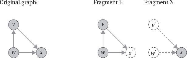
Moreover, whenever a graph query traverses an edge between two vertices that are located on two different servers, the graph database must quickly identify the second server that hosts the corresponding second vertex. In this case, shadow nodes (and corresponding shadow edges) are maintained as shown in Figure 11.2 that enable fast traversal between fragments.

11.2.4 Sharding for Key-Based Stores

Data stores with key-based access include not only key-value stores but also document databases (where the document ID is the key) and column-family stores (by using the row key). In other words, the basic way to interact with key-based data store is to send a query containing the key, and then the data store identifies the record corresponding to the key and returns this record. These key-based stores rarely support operators that combine different records; this is in contrast to relational databases that support join operations. Consequently, when fragmenting data in key-based stores the fragments require less interconnection between the fragments and fragments can be stored independently on different servers. The term used for this kind of fragmentation in key-based stores is sharding. Sharding is similar to horizontal fragmentation for relational databases in the sense that it may be used to split a dataset into individual data records like rows or documents. However, the term sharding also connotes that the shards can be schemaless (as can be the entire set of records in the data store). In particular, these data stores do not support general value-based fragmentation (based on a selection operation on values inside the data records); they only support range-based or hash-based fragmentation for the keys. Moreover, there is no need to support derived fragmentation due to the lack of a join operation.

Some stores order the records by key. In this case, order-preserving partitioning of the records may be applied: the order on the keys provides semantic information on how related the records are; when two keys are close in the order defined on the keys, then they are also closely related and are often accessed by the same client. However, order-preserving partitioning may lead to hotspots when one partition is prone to more excessive accesses than other partitions.

11.2.5 Object Fragmentation

Following the terminology of the relational fragmentation, some approaches [KL00] define vertical and horizontal fragmentation for object-oriented programs. In this case, either a single object can be fragmented into subobjects – this corresponds to a structure-based fragmentation because new class definitions for the subobjects have to be specified; or the set of objects is fragmented into subsets of objects as a value-based fragmentation. Alternatively, as third and most viable option, the entire object graph (the virtual heap; see Chapter 9) can be fragmented into subsets of objects. We briefly sketch these different approaches and leave further elaboration as an exercise.

1.Vertical fragmentation of single objects splits an object into two or more objects. Each of the new objects contains a subset of the original object’s variables. Then the class definition has to be split, too, into several classes. The advantage would then be that when accessing the object not the entire set of its variables must be loaded from the database but only one subset. This notion of vertical fragmentation can however be criticized: it contradicts the object-oriented paradigm of encapsulation because it breaks the object boundaries. With a good design and a good normalization of the program, objects should represent an entity and encapsulate all the necessary state and behavior; hence objects should not be fragmented any further.

2.Horizontal fragmentation of the object graph. The set of instances of a class can be fragmented into subsets. This can for example be based on the value of some instance variables: a set of objects representing employees of different companies can be fragmented into subsets for employees of each of the individual companies. Or the fragmentation can be affinity-based by identifying a subset of objects that are often accesses together. A derived horizontal fragmentation is also possible: those objects of other classes can be fragmented based on the fact with which objects in a horizontal fragment they interact or which objects are referenced by them.

3.Graph partitioning algorithms (see Section 11.2.3) can also be applied to the virtual heap. A minimum edge cut partitioning of the virtual heap would then group those objects together that are highly connected by edges (representing references or associations) between them. Edges in the object graph can occur due to direct referencing of another object but also indirectly due to the class hierarchy (that is, the inheritance relation between objects).

11.3 Data Allocation

For fragmented data a major problem is how to distribute the fragments over the database servers; a data allocation mechanism has to decide which fragment should be stored on which server. As an important side effect of data allocation, load balancing has to be taken into account: fragments should ideally be distributed evenly across all servers. There are several forms of data allocation:

Range-based allocation relies on range-based fragmentation (see Section 11.1): When a range-based fragmentation is obtained (for example, order-preserving partitioning of key-based stores), the identified ranges have to be assigned to the available servers. This range-based allocation might have an adverse effect on load balancing: because the entire set of possible records is split into ranges, the majority of actual records in the database might be located only in some few ranges (while for the other ranges there are no or just few records contained in the database). Servers getting assigned the more populated ranges hence have higher load. But even if ranges are more or less equally populated, the load balancing depends also on the query patterns that occur: if records in one range are accessed more often than those in other ranges, the server having this range has more processing load than the others. That is, this server becomes a hot spot and is more prone to delaying or failing.

Hash-based allocation uses a hash function (like MD5 or MurmurHash) over the input fragments to determine the server to which each fragment is assigned. In this case, ranges for the servers are defined on the set of output values of the hash function. Even with hash-based allocation, hotspots can occur because some records on one server are accessed more often than the ones on other servers; however, with hash-based allocation the distribution of the records among the servers is usually more balanced because the hash function distributes its input values well over its entire output hash values. For key-based stores, hash-based allocation is often used in conjunction with hash-based fragmentation (see Section 11.1): that is, for key-based access, first the hash function is computed on the key of each record; then – depending on the range in which this hash value lies – the corresponding server is determined. This hash value must then also be computed when a key is queried to determine the server on which the key is located. Consistent hashing as a popular form of hash-based allocation is presented in detail in Section 11.3.2.

Cost-based allocation describes the data allocation task as an optimization problem. The cost model can take several parameters into account; for instance, two important parameters are minimizing the amount of occupied servers and minimizing the amount of transferred data. A more detailed discussion is provided in Section 11.3.1.

11.3.1 Cost-based allocation

Cost-based allocation can be seen as a combinatorial optimization problem with several parameters where the goal is to minimize a cost function. The optimization problem can be expressed by a so-called integer linear program (ILP).

More formally, the data distribution problem is a description of the task of distributing database fragments among a set of servers in a distributed database system. The data distribution problem is basically a Bin Packing Problem (BPP) in the following sense:

–K servers correspond to K bins

–bins have a maximum capacity W

–n fragments correspond to n objects

–each object has a weight (in other words a size or a capacity consumption) w_i≤W

–objects have to be placed into a minimum number of bins without exceeding the maximum capacity

This BPP can be written as an integer linear program (ILP) as follows – where x_ik is a binary variable that denotes whether fragment/object i is placed in server/bin k; and y_k denotes that server/bin k is used (that is, is non-empty):

To explain, Equation 11.1 means that we want to minimize the number of servers (that is, bins) used; Equation 11.2 means that each object is assigned to exactly one bin; Equation 11.3 means that the capacity of each server is not exceeded; and the last two equations denote that the variables are binary – that is, the ILP is a so-called 0-1 linear program. When solving this optimization problem, the resulting assignment of the x-variables represents an assignment of fragments to a minimum amount servers.

While in this simple example only the storage capacity (W) of the servers and the storage consumption (w_i) of each fragment are considered, in general other cost factors can be included when calculating an optimal allocation with minimal cost. For example, as additional background information, a typical workload can be considered and data locality of fragment allocation can be improved; in this way, network transmission cost is reduced because less servers have to be contacted when evaluating queries from the workload.

11.3.2 Consistent Hashing

Due to the danger of hotspots, consistent hashing as a form of hash-based allocation is usually preferred. It provides a better and more flexible distribution of the records among a set of servers. It originates from work on distributed caching [KLL+97]; it has later been popularized for data allocation by the Dynamo system [DHJ+07] and now is widely applied by distributed database systems to allow data allocation that tolerates churn in the network (that is, adding or removing database servers).

As consistent hashing is a hash-based allocation scheme, a hash function is computed on each input fragment. The first essential concept of consistent hashing is that the hash values are now seen as a ring that wraps around: when we have reached the highest hash value we start again from 0. The second essential concept is that a hash value is computed not only for each fragment but also for each database server (for example by taking the hash of the server name or IP address).

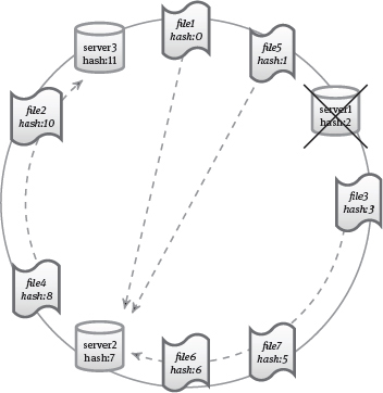
By computing a hash value for a database server, each server has a fixed position on the ring; the advantage of these hash values is that they presumably distribute the servers evenly on the ring (if the hash function has good distribution properties). Similarly for each data item a hash value is computed – for example the hash of the key of a key-value pair. In this way, data also distribute well on the ring. A widely used allocation policy is then to store data on the next server on the ring when looking in clockwise direction; this is illustrated in Figure 11.3.

A major advantage of consistent hashing is its flexible support of additions or removals of servers. Whenever a server leaves the hash ring, all the data that it stores have to be moved to the next server in clockwise direction (see Figure 11.4). Whenever a server joins the ring, the data with a hash value less than the hash value of the new server have to be moved to the new server; and they can then be deleted from the server where they were previously located – that is, the next server in clockwise direction (see Figure 11.5).

An important tool to make consistent hashing more flexible is to have not only one location on the ring for each physical server but instead to have multiple locations: these locations are then called virtual servers. Virtual servers improve consistent hashing in the following cases:

–The virtual servers (of each physical server) are spread along the ring in an arbitrary fashion and virtual servers of different physical servers may be interleaved on the ring. In this way, all servers have a better spread on the ring; this leads to a more even data distribution among the servers on average.

–Heterogeneous servers are supported: a server with less capacity can be represented by less virtual servers than a server with more capacity. In this way the weaker server has to handle less load than the stronger server.

–New servers can be gradually added to the ring: instead of shifting its entire data load onto a new server at once, virtual servers for the new server can be added one at a time. In this way the new server has time to start up slowly and take on its full load step by step until its full capacity is reached.

In many implementations, the hash ring is divided into several ranges of equal size. Each server is assigned a subset of these ranges. Whenever servers join or leave the network, the ranges get reassigned.

11.4 Bibliographic Notes

Fragmentation and allocation for relational databases is extensively discussed in [ÖV11].

Ma and Schewe [MS10] discusses both vertical and horizontal fragmentation for both object-oriented and XML data and introduces the notion of a split fragmentation. Horizontal or vertical fragmentation of XML documents while improving query processing has been studied by several authors including [KÖD10, FBM10, ARB+06].

For graphs usually a minimum edge cut partitioning is obtained. The influential article by Karypis and Kumar [KK98] describes a graph partitioning algorithm with a coarsening, a partitioning and an uncoarsening phase. Dynamic changes in graphs can be handled by the xDGP system of Vaquero et al. [VCLM13] by vertex migration. With a particular focus on graph partitioning for graph databases, Averbuch and Neumann present a graph partitioning algorithm that can adapt to graph changes and an implementation and evaluation with the Neo4J graph database.

Consistent hashing was first used for distributed caching [KLL+97] and has later on been widely applied for peer-to-peer systems like distributed hash tables – for example in [SMK+01]. It has then been applied to data fragmentation and allocation in key-value stores [DHJ+07] as well as document stores and extensible record stores.