
11
Moire Fringes Technique
11.1 INTRODUCTION
Moire is a French word and its meaning is watered silk, which is a common optical phenomenon being observed daily if a fold of silk or any other finely woven fabric is allowed to slip on another fold and viewed against a light background simmering zig-zag patterns, localized between two folds of fabric. Such patterns are also seen in mismatched window blinds or superimposed fine wire meshes. In other words, whenever a geometric figure repeating itself regularly such as a set of straight lines, dots, meshes, etc. is superimposed on another similar but not of identical pattern, moire fringes are visible.
Initially moire fringe effect was a problem and needed to be eliminated because these fringes were due to errors in spacing, parallelism, and straightness of lines in rulings used for diffraction gratings. But now the technique has found innumerable applications wherever a precise measurement of relative movement is required such as in machine tool control, metrology, strain analysis, and study of dislocations in crystals. The simple obstruction theory of light in which an opacity in one grid obstructs the light from the transparency in the other grid explains the formations of fringes.
11.2 STRAIN ANALYSIS THROUGH MOIRE FRINGES
In this technique, a grid is fixed on the surface of the model to be analysed for strains. When the load is applied on the model, the grid on the model called the model grid is deformed. If another grid, similar to the undeformed model grid, and called the master grid, is placed in front of the deformed (or strained) model grid and light is allowed to pass through, fringes are visible in the field of view. These fringes are called ‘moire fringes’ and can be used to compute the strains at various points of the model. It is usual to use grids consisting of equally spaced straight parallel non-diffracting lines though grids from circular, radial, or other non-parallel arrays can also be used for the formation of Moire fringes.
The moire technique for strain measurement is ideally suited for the measurement of strains greater than or equal to 200 microstrain.
For the analysis of moire fringe pattern to calculate strains in model, two distinct approaches can be used, i.e. (i) geometrical approach and (ii) displacement approach. In the geometrical approach, fringe pattern is regarded as the result of intersections of the rulings of the model grid and master grid. Considering the geometry of the fringe pattern, it is possible to deduce expressions for the distance between the model grid lines and the change in their direction caused by strain in terms of the pitch of lines on master grid and the fringe characteristics. The measurement of fringe characteristics such as their separation and inclination of the master grid lines enables one to compute the normal and shear strains at the point of observation.
In displacement approach, moire fringe pattern is used for determining displacements. Consider, for example, a simple tension test specimen with a line grid fixed on it and let a simple uniform tension be applied to the test specimen in a direction normal to the grid lines. The applied tension will change the pitch of the model grid. If another grid with the same pitch as the unstretched model grid be superimposed on it, a series of bright and dark fringes will be seen in the field of view.
Figure 11.1 shows the formation of dark and bright fringes. We have bright fringes at A, C, and E and dark fringes at B and D.
The distance between the centres of the two consecutive bright or dark fringes is equal to the master pitch divided by strain. The fringes can thus be considered as the loci of the points of equal displacement in a direction normal to the rulings. No doubt a simple uniaxial tension test piece is considered but the argument can be extended to a general strain field and the moire fringes can be considered as the loci of points of constant displacement. Measurement on these fringes gives us the displacement in x and y directions and strains εxx, εyy, γxy are calculated from these displacements in a usual manner.
Now the model grid is fixed to the structure or a component under investigation. The master grid is used as a reference grid (i) for the purpose of producing and analyzing moire pattern and (ii) establishing directions of the co-ordinate axes.
The distance between points of any two consecutive ruling on the master grid is called master pitch, p. The direction perpendicular to the ruling and lying in the plane of master grid is known as principal direction and is denoted by r. The direction parallel to the ruling is often called the secondary direction and is denoted by s.
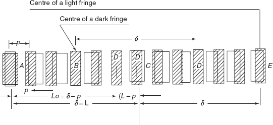
Figure 11.1 Light and dark moire fringe tension or compression
The model grid undergoes the same deformation as the model itself because it is fixed to the model. Therefore, after the model is loaded, the pitch of the model grid changes from point to point. Say the model grid pitch in any deformed state is p′. The centre-to-centre separation between any two consecutive dark or bright fringes is called the inter-fringe. Say the interfringe between two closely spaced fringes measured along the normal to the fringe is denoted by δ (See Figure 11.1). Sometimes it is more convenient to measure the interfringe along r and s directions. In such case, distances are denoted by δr, and δs, respectively.
11.3 GEOMETRICAL APPROACH
- Pure normal strains perpendicular to grid lines: Consider the ideal case of a test specimen subjected to uniaxial tension along the principal direction r. The master grid is superimposed over model grid without any rotation. On account of normal strain, the pitch of the model grid is changed and the ruling on the model and master grids are no longer in alignment, consequently bright and dark fringes are formed and are visible in the field of view.
Say n = number of lines on the reference grid between two successive bright or dark fringes.
Then n – 1 = number of lines on the model grid between two successive bright or dark fringes (if test piece is in tension)
or n + 1 = number of lines on the model grid between two successive bright or dark fringes, if test piece is in compression.
Then
δ = np = (n − 1)p′
(11.1)
Moreover
δ = (n − 1)p (1 + εxx),
(11.2)
where δ is interfringe spacing.
From these equations

In the elastic region
 , therefore (on the case of tension)
Similarly in the case of compression

or
From Eq. (11.3) we can determine strain εxx knowing the value of master pitch p and measuring the interfringe spacing δ.
- Pure rotation: To obtain an expression for the relative orientation in terms of the fringe spacing and the grid pitch, let us consider two line grids of identical pitch p, making a small angle as shown in Figure 11.2. It is obvious that the diagonal AB of the rhombus is formed by two pairs of grid lines from the geometry of the figure, we can write
or
For small value of θ < 10°,
 . Thus Eq. (11.4) enables us to calculate θ from the measured values of δ, interfringe spacing:
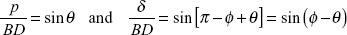
 - Combined shear and normal strains (or rotation and stretching/contraction): Say the acute angle measured from the fixed master grid lines to the model grid lines is denoted by θ. The angle measured from the fixed master grid lines to a fringe at a point in the direction of θ is designated by ϕ. This angle ϕ can be acute or obtuse. Let B be the point of observation. The master grid lines with pitch p are shown. The model grid lines with pitch p′ are also shown. The resulting moire fringes are shown by thick lines. The angles θ and ϕ are shown in Figure 11.3. In this case ϕ is an obtuse angle.
ϕ = ∠ EBD angle made by the model grid line with the master grid line.
ϕ = ∠ EBA = angle measured from the fixed master grid line to a moire fringe at the point B in the direction of θ.
ϕ = ∠ EBA = angle measured from the fixed master grid line to a moiré fringe at the point in the direction of θ.
δ = BF = interfringe spacing.
Now
or
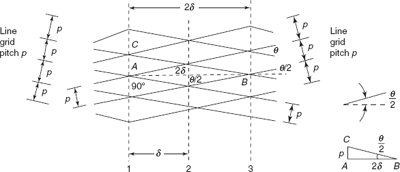

Figure 11.3
or
or
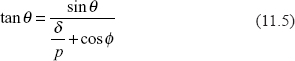
Since p is known and δ and ϕ can be measured, rotation θ can be calculated from Eq. (11.5).
If gratings with a very fine pitch are used to measure small angles of rotation, then ![]() . Eq. (11.5) reduces to
. Eq. (11.5) reduces to
or ![]()
Now |
DE = p, pitch of master grid |
|
DK = p′, pitch of deformed model grid |
It is also observed that
or ![]()
Thus ![]()
But from Eq. (11.5)
Substituting the value of sin(ϕ − θ) in Eq. (11.7), we get
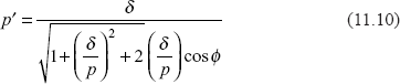
Moreover, ![]()
Therefore
Now substituting the value of  in Eq. (11.9) we can write
Langrangian strain in the direction r
Eulerian strain the direction r will be
11.4 DISPLACEMENT APPROACH
A moire fringe is a locus of points having the same magnitude of displacements in the principal direction of master grating. Such a locus is called an isothetic. Therefore, a moire fringe, an isothetic pattern, can be visualized as a displacement surface where the height of a point on the surface above a reference plane represents the displacement of the point in the principal direction of master grating. Two isothetic patterns are obtained using line gratings perpendicular to x-axis and y-axis, respectively, on the surface of a specimen under investigation. From these moire gratings u and v displacements are determined by noting down the order of fringes Nx and Ny.
Then
|
u = Nx p |
|
|
v = Ny p |
(11.11) |
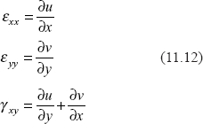
The Cartesian components of strain can be computed from the derivatives of displacements as follows:
The slopes of displacements as above are obtained by drawing tangents to the displacement curves of u and v fields along x and y axes.
Figure 11.4(a) shows the moire fringes when the model grating is perpendicular to x-axis. Order of the fringes Nx, are marked (–3 to + 4) as shown.
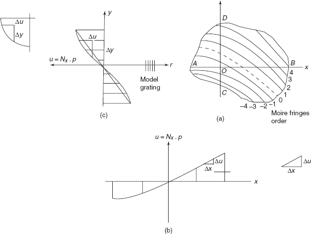
Figure 11.4 The moire fringes when the model grating is perpendicular to x-axis
Lines along x and y axes say AB and CD are drawn. The displacement u along AB and CD are plotted by noting that u = Nx., p, where p is the pitch of master grating.
Now Figure 11.5(a) shows the moire fringes when the model grating is perpendicular to y-axis. Order of the fringes Ny are marked (–2 to + 6) as shown in Figure 11.5(a). Lines AB and CD along x and y axes are drawn. The displacement v along AB and CD is plotted by noting that v = Ny. p where p is the pitch of the master grating. From the plots of u versus x, u versus y, v versus x, and v versus y, strains at any point are determined by using the relationships given by Eqs (11.12).
Problem 11.1 Two gratings of density 25 line per mm are used for strain analysis in a uniform strain field of uniaxial tensile strain. If the distance between the fringes is uniform all over the field and equal to 3.6 mm, determine the Eulerian and Langrangian strains. What would be the strains if it were a compressive strain field?
Solution: Master grating pitch, ![]()
Interfringe spacing, δ = 3.6 mm
n = number of lines on the reference grid between successive bright or dark fringes.
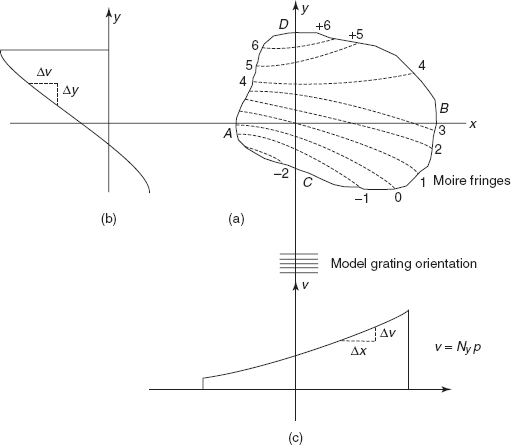
Figure 11.5
- Uniaxial tensile strain
Number of lines on the model grid between two successive bright or dark fringes
= n − 1 = 90 − 1 = 89Pitch on model grid, p′ = 3600/89 = 40.45 micron
Langrangian strain,
Eulerian strain
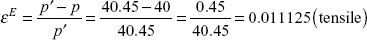
- Uniaxial compressive strain
n = 90
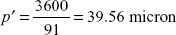
n + 1 = 90 + 1 = 91, number of lines of the model grid between two successive bright or dark moire fringes
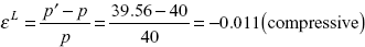
Model grid pitch,
Langrangian strain,
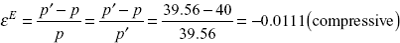
Eulerian strain,
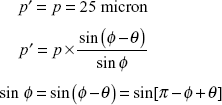
Problem 11.2 When a grating of pitch 40 lines per mm is given a slight rotation θ with respect to a second grating of the same pitch, moire fringes are formed making an angle ϕ with respect to second grating. Determine the angle θ and interfringe spacing δ, if the angle ϕ is equal to (i) 60° and (ii) 110°.
Solution: Master grating pitch,
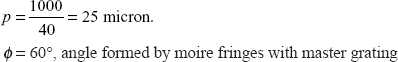
Model grating pitch,
|
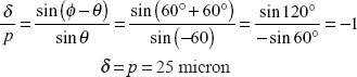
ϕ = 60° |
So, |
ϕ = π − ϕ + θ |
Angle of rotation,
Moreover,
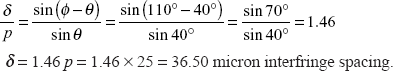
(ii)
ϕ = 110°
sinϕ = sin(ϕ − θ), because p = p′
sinϕ = sin(π − ϕ + θ)also
ϕ = π − ϕ + θ
2 ϕ − π = θ
2 × 110° − 180° = θ
θ = 40°, angle of rotation.
Now,
Multiple choice QUESTIONS
- If two gratings of density 25 lines per mm are used for strain’ analysis in a uniform strain field and distance between fringes is observed as 36 mm, what is the order of strain?
- 900 μ strain
- 1000 μ strain
- 1110 μ strain
- None of these
- When a grating of pitch 40 lines per mm is given a slight rotation θ with respect to a second grating of same pitch, moire fringes are formed making an angle of 70° with respect to second gratings. What is angle θ?
- –60°
- –50°
- –40°
- None of these
- If pitch on master grating is p and pitch on model grating is p′ (initially both pitches are the same) due to strain p changes to p′ on model grating. What is Eulerian strain?


- None of these
- In pure rotation case, if pitch p = 40 microns, and δ = 1 mm (fringe spacing), what is angular rotation θ?
- 3°
- 2.3°
- 2°
- none of these
Answers
1. (c) |
2. (c) |
3. (a) |
4. (b) |
|
PRACTICE PROBLEMS
11.1 Two gratings of density 32 lines per mm are used for strain analysis in a uniform strain field of uniaxial tensile strain. If the distance between the fringes is uniform all over the field and equal to 4 mm, determine the Eulerian and Langrangian strains. What would be the strains if it were a compressive strain field
Ans. [7.874 × 10⁻¹, 7.81 × 10⁻¹, −7.7536 × 10⁻¹, −7.814 × 10⁻³].
11.2 When a grating of pitch 32 lines per mm is given a slight rotation θ with respect to a second grating of the same pitch, moire fringes are formed making an angle of ϕ with respect to second grating. Determine the angle θ and interfringe’ spacing δ if angle ϕ is equal to (i) 70° and (ii) 100°.
Ans. [−40°, 45.7 micron, + 20°, 90 micron].