
2
Mechanical Behaviour of Materials
2.1 INTRODUCTION
Behaviour of a material against mechanical loading is an important consideration for a designer while designing a structural member or a machine member. A specimen of a material is tested under tensile loading to determine yield strength, ultimate strength, and ductility of the material. Toughness is another important mechanical property of materials which is obtained by notched bar import test. Similarly, the resistance of the material to wear and tear during operation is tested by a hardness test. Many engineering materials are subjected to reversed stress cycles, such as springs, aircraft wings, blades of a turbine, rotating shafts, and such components are tested under fatigue loading and fatigue behaviour is ascertained by standard fatigue tests. Yet there are many components which deform with time under constant stress such as blades of a gas turbine, beds of furnaces, etc.; such components are tested under constant load to analyze their creep behaviour.
2.2 CRYSTALLINE MATERIALS
Most of the metals are polycrystalline materials, in which the crystals are randomly oriented. A crystal is a three-dimensional structure containing unit lattices of atoms, in which atoms are arranged in a specific order. Each lattice has slip planes of maximum atomic density, along which the atoms can slip easily during the plastic deformation of the crystal. Figure 2.1 shows parallel lines of slip planes (or crystallographic planes of maximum atomic density). All the crystals are randomly distributed, i.e. their slip planes do not have any preferential direction as shown.
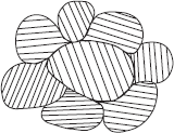
Figure 2.1 Polycrystalline material
Most common atomic arrangements in metals are body centred cubic (BCC), face centred cubic (FCC), and hexagonal close packed (HCP) as shown in Figure 2.2.
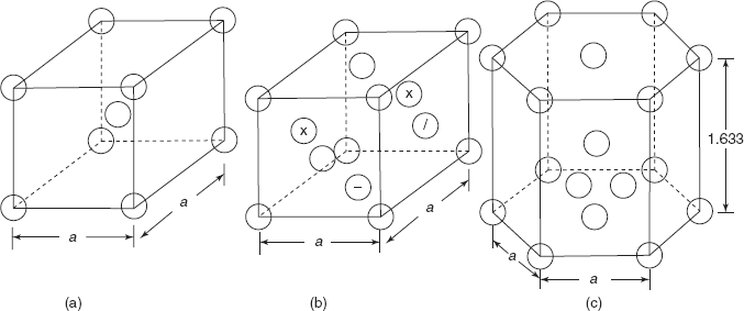
Figure 2.2 (a) Bcc structure (b) Fcc structure (c) hexagonal closed packed structure
Figure 2.2(a) shows a BCC structure, in which eight atoms are arranged on eight corners of cube and one atom is located in the body centre of cube. Figure 2.2(b) shows an FCC structure in which eight atoms are located on eight corners of cube and six atoms are located at the centre of six faces of cube. Similarly, Figure 2.2(c) shows a hexagonal closed packed structure in which there are six atoms on above hexagonal plane, one atom at the centre of hexagonal plane, and similarly seven atoms in the lower hexagonal plane. Then there are three atoms arranged in the centre of the body of HCP system. The atoms are not so small as shown in Figure 2.2, rather these atoms of spherical shape touch each other. One atom at the corner of a BCC system is shared by eight unit lattices meeting at the point. So, in all there are ![]() atoms in a BCC structure.
atoms in a BCC structure.
In FCC structures, each atom at the corner of cube is shared by eight adjoining unit lattices and each atom of face is shared by another unit lattice also. So, overall there are ![]() atoms per FCC unit lattice.
atoms per FCC unit lattice.
In HCP, each corner atom is showed by six unit lattices and each atom at centre of hexagonal face is shared by another unit lattice also. So, in effect there are ![]() atoms in HCP unit lattice.
atoms in HCP unit lattice.
Moreover in BCC, each atom is touched by eight adjoining atoms, in FCC each atom is touched by 12 adjoining atoms and in HCP each atom is touched by 12 adjoining atoms (say central atom on hexagonal plane is touched by six atoms on the same plane, then it is touched by three central atoms of upper lattice and three central atoms of lower lattice. So, in HCP each atom is surrounded by 12 atoms. Therefore, co-ordination number of a BCC structure is eight, of an FCC structure, it is 12 and of an HCP structure it is 12.
Let us now determine the radius of the atom in terms of the side of the cube in BCC, FCC, and the side of hexagonal in case of HCP.
Knowing the radius of atom in terms of lattice parameter a, we can find the volume of two atoms in a BCC structure, four atoms in an FCC structure and six atoms in an HCP structure (Figure 2.3).
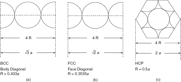
Figure 2.3 Relation between atomic radius and lattice parameter
Atomic packing factor,
Reader can do this exercise to find out that packing factor for a BCC structure is 0.68, for an FCC structure it is 0.74, and again for HCP structure APF is 0.74.
It is needless to mention that the mechanical properties of a material, such as ductility, strength, depend on the crystal structure of a material.
2.3 CRYSTAL STRUCTURES OF VARIOUS ELEMENTS
For various elements, atomic radius is nm and the crystal structure is given in Table 2.1.
It can be noted that for most of the metallic elements (except lead) atomic radius is less than 0.15 nm. Carbon is an impurity atom and takes interstitial position in an FCC structure of γ iron and produces hard and strong cementite. Moreover, it occupies interstitial position in BCT (body centred tetragonal structure where sides are a, a, c > a) and produces hard and brittle martensite.
In a BCC structure, there is hardly any space available for small carbon atoms to take interstitial position. Therefore, in a BCC structure at the room temperature the maximum solubility of carbon in iron is only 0.008%. But in an FCC structure there is available space for interstitial position of small carbon atoms and carbon up to 2.1% is soluble in γ iron, i.e. of FCC structure (Figure 2.4b). In the BCT structure (body centred tetragonal), one side of cube is elongated c > a, making space available for interstitial position of carbon in iron atoms.
In martensite carbon atoms are easily absorbed and martensite is the supersaturated solid solution of carbon in iron. Martensite structure is very hard and brittle, useful for cutting tools.
Table 2.1 Crystal structure of various elements
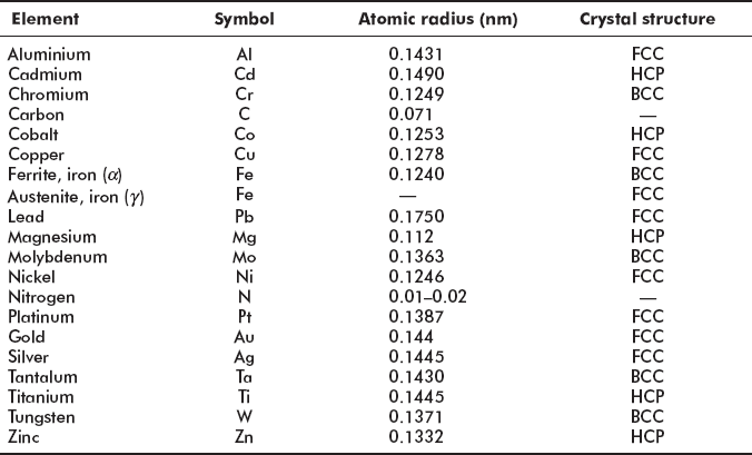
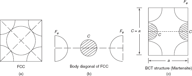
Figure 2.4 Different crystal structures
2.4 ATOMIC BONDING
Figure 2.5 shows two isolated atoms of a solid. Bonding between two atoms is illustrated by interatomic forces between two atoms, i.e. attractive force between protons and electron and repulsive force between protons of two atoms.
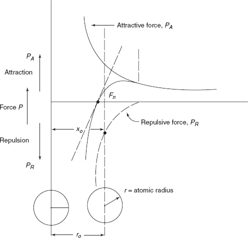
Figure 2.5 Graph between force and interatomic distance
At large distances interatomic forces are negligible.
Net force between two atoms
|
PN |
= |
PA + PR |
|
|
= |
0 for a state of equilibrium |
Equilibrium spacing, x0 = 0.3 nm (3Å) for many atoms. In this equilibrium position, the two atoms will counteract any attempt to separate them by an attractive force; similarly an attempt to push them together is resisted by repulsive force PR. There forces PA and PR depend upon the type of bonding existing between two atoms.
Potential energy between the two atoms can be expressed as
Net potential energy |
= |
Attractive energy + repulsive energy between two atoms |
U0 |
= |
Bonding energy of the two atoms correspond to the energy at the position of equilibrium when the distance between two atoms is x0 |
Many material properties depend on U0, enumerated as follows:
- Materials having large bonding energies also have high melting point.
- At room temperature, solid substances are formed for large bonding energies.
- For gaseous state, small energy is required.
- Liquids possess medium potential energy.
- Young’s modulus or stiffness of a material is dependent on the shape of Net force versus interatomic spacing curve, slope of curve at x0 defines E, as shown in Figure 2.5, by tangent at the curve at x0.
- Coefficient of thermal expansion depends on bonding energy U0.
2.4.1 Metallic Bonding
Metallic materials have one-, two-, or at the most three-valency electrons. These valency electrons are not bound to any particular atom in the solid, and they are free to drift throughout the solid. These valency electrons form a cloud of electrons around atoms. The remaining non-valency electrons and atomic nuclei form ion cores, which possess a net positive charge equal in magnitude to the total valency electrons charge per atom. The free electrons shield the positively charged ion cores from mutually repulsive electrostatic forces. Free electrons act as binding adhesive to hold ion cores together. Metals are good conductors of heat and electricity both; it is due to the presence of free electrons as shown in Figure 2.6.
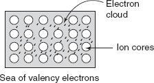
Figure 2.6 Metallic bond
2.5 SINGLE CRYSTAL
When the periodic and repeated arrangement of atoms (as in unit lattices) is perfect and extends throughout the volume of specimen, without any interruption, the result is a single crystal. Although single crystals exist in nature, they may be produced artificially. If the boundaries of single crystal are allowed to grow without any external constraint, the crystal will assume a regular geometric shape as in gem stones. In electronic microcircuits, single crystals of silicon and germanium are extensively used.
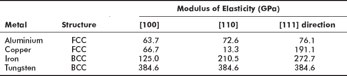
The physical properties of a single crystal depend on crystallographic direction in which measurements are taken, as is obvious from Table 2.2.
Table 2.2 Effect of crystallographic directions on Young’s modulus of metals
2.6 POLYCRYSTALLINE MATERIALS
Most crystalline solids are composed of a collection of many small crystals or grains and such materials are termed as polycrystalline. From molten state there are various stages of solidification as (a) small nuclei form on various positions, having random crystallographic orientation, (b) small grains grow by successive addition of atoms from surrounding liquid, (c) extremeties of adjacent grains impinge on one another as the solidification process approaches completion.
For many polycrystalline materials, the crystallographic orientation of individual grains is totally random and each grain is anisotropic, because the physical properties depend on the crystallographic direction in which measurements are taken, yet the specimen composed of the grain aggregate behave isotropically representing the average of directional values.
2.7 IMPERFECTIONS IN SOLIDS
An idealized solid with a perfect order existing throughout the crystalline material does not exist; all materials contain large number of various defects and imperfections, and mechanical properties of any material are profoundly influenced by the presence of these imperfections. The crystalline imperfections can be classified as (i) point defects (associated with one or two atomic positions), (ii) linear defect or one-dimensional defect, and (iii) interfacial defects or grain boundaries—termed as two-dimensional impurities.
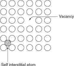
Figure 2.7 Point imperfections
Equilibrium number of vacancies is
where |
N |
= |
total number of atomic sites, |
|
QV |
= |
energy required for the formation of one vacancy, |
|
k |
= |
Boltzman constant, 1.38 × 10⁻²³ J/atom-K, and |
|
T |
= |
absolute temperature in °K. |
A self-interstitial atom is crowded into an interstitial site, a small void smaller than the size of an atom, so self-interstitial atom produces large distortion in a crystal. The formation of this defect is highly improbable but vacancies are common. For most metals, the fraction of vacancies Ne /N just below the melting temperature is of the order of 10–4.
2.7.1 Impurities in Solids
Impurity or foreign atoms will always be present in metals. Most familiar metals are not highly pure; rather they are alloys in which impurity atoms have been intentionally added to impart specific characteristics to the material. The addition of impurity atoms to a metal will result in the formation of a solid solution and/or a new second phase, depending on the type of impurity.
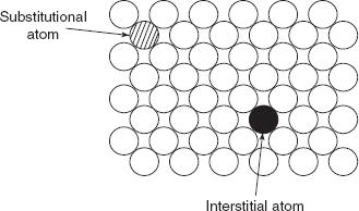
Figure 2.8 Impurities in solids
A solid solution is formed when some solute atoms are added to the host material (solvent), the crystal structure is maintained, and no new structures are formed. The impurity atoms are randomly and uniformly dispersed with the solid.
Figure 2.8 shows (i) substitutional solid solution of atoms of the same size and (ii) interstitial solid solution of smaller atom.
Copper and nickel make perfect solid solution because both have FCC structures, and their atomic radius is 0.128 nm and 0.125, respectively.
In iron and carbon, i.e. steel, carbon atom occupies interstitial position because carbon atom is smaller than iron atom; the atomic radius of iron atom is 0.124 nm while the atomic radius of carbon atom is 0.071 nm.
2.8 DISLOCATIONS
A dislocation is a linear defect, i.e. one-dimensional defect around which some of the atoms are misaligned or displaced from normal configuration. Figure 2.9 shows an extra plane of atoms ABCD squeezed into the three-dimensional network of unit lattices, during the mechanical deformation of a body. Just above the edge AB, an extra incomplete plane of atoms ABCD squeezed together and atoms on this plane are in a state of compression, i.e. distance r < x0 (less than the interatomic spacing for equilibrium). Below the edge AB, atoms are pulled apart r′ > x0 and atoms are in a state of tension. The distorted configuration extends all along the dislocation edge AB in the crystal. The potential energy increases for an increase in bond length r′ > x0 as well as for decrease in bond length r < x0. There is extra strain energy due to the distortion in the region surrounding the edge of incomplete plane ABCD.
As the region of maximum distortion is centred around the edge of the incomplete plane, this distortion represents a line imperfection and is called an edge dislocation. Depending upon the location of incomplete plane, i.e. starting from top or starting from bottom of the crystal, the two configurations are known as positive and negative edge dislocations, respectively, and are represented by ⊥ and ┬ symbols. Plane EAF is known as slip plane. Region over the slip plane is called slipped part and region below the slip plane is called unslipped part. Plane EAF is the boundary between slipped and unslipped parts.
2.8.1 Burger’s Vector
The direction and magnitude of an edge dislocation are determined by a vector called Burger’s vector, and it can be known on drawing a Burger’s circuit. In Figure 2.9, a circuit starts from a, going up by five steps, circuit goes towards right from b to c, six steps, then coming down by cd, by five steps and then moving towards left by six steps, the circuit is completed at a′. The unclosed side aa′ is called Burger’s Vector. In an ideal crystal with no edge dislocation, Burger’s vector |b| = 0. In imperfect crystal Burger’s vector is |b| = a, space lattice unit. Burger’s circuit has been drawn clockwise, viewing along the direction ![]() of edge dislocation. Burger vector aa′ is perpendicular to edge dislocation AB.
of edge dislocation. Burger vector aa′ is perpendicular to edge dislocation AB.
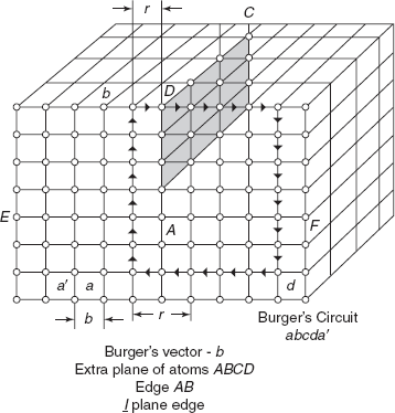
Figure 2.9 Edge dislocation
2.8.2 Screw Dislocation
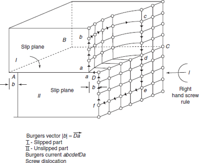
There is no extra plane in the case of screw dislocation in crystal. When part of the crystal displaces angularly with respect to the other part, a screw dislocation is formed, as if a shear stress has produced this dislocation. Angular displacement is similar to a screw movement; therefore, this angular displacement is termed as screw dislocation. Symbolically screw displacement is represented by ![]() or
or ![]() and are referred to as positive and negative screw dislocations. Figure 2.10 shows screw dislocation, in which Part I of crystal slips angularly over Part II of crystal along the slip plane ABCD. Line dD is slipped to new position da. Dislocation has occurred along slip plane ABCD. Screw dislocation line l is marked in the direction of arrow l. The atomic bonds in the vicinity of dislocation line undergo shear deformation, developing shear stress and shear strain field.
and are referred to as positive and negative screw dislocations. Figure 2.10 shows screw dislocation, in which Part I of crystal slips angularly over Part II of crystal along the slip plane ABCD. Line dD is slipped to new position da. Dislocation has occurred along slip plane ABCD. Screw dislocation line l is marked in the direction of arrow l. The atomic bonds in the vicinity of dislocation line undergo shear deformation, developing shear stress and shear strain field.
If we draw Burger’s circuit from point a, moving three steps upwards by ab and moving four steps towards right along bc and coming down by six steps along cde, then moving four steps towards left by ef, then going up by three steps up to D, by f D, then ![]() is the closing side of the circuit, giving Burger’s vector |b| which is parallel to screw dislocation line l as shown.
is the closing side of the circuit, giving Burger’s vector |b| which is parallel to screw dislocation line l as shown.
Dislocations having mixed character, i.e. combining edge and screw dislocations, are termed as mixed dislocations. When extra plane of atom is accompanied by angular twist of slipped part, the consequence is a mixed dislocation. Mixed dislocations generally emerge at the curved boundary on which directional continuity changes as in the case of holes, notches, etc.
2.8.3 Characteristics of Dislocations
Properties and behaviour of dislocations are briefly described as follows:
- A crystal normally incorporates large number of dislocations. So, there exist numerous Burger’s vectors. The sum of these Burger’s vectors meeting at a point called a nodal point is zero.
- A dislocation does not end abruptly with in the crystal; it vanishes either at the nodal point or on the surface of the crystal.
- A dislocation under the influence of stress field may close on as a loop. The profile of the loop may be a circle or an edge.
- Distortional energy is produced in dislocation due to tensile and compressive stress–strain field in edge dislocation and due to shear stress–shear strain field in screw dislocation.
- Elastic strain energy per unit length of dislocation is
 where G is the shear modulus and b is Burger’s vector.
 - Dislocations have inherent tendency to keep smallest Burger’s vector, which increases stability of crystal.
- Two edge dislocations of opposite sign ⊥ and ┲ of equal Burger’s vector cancel out each other.
- Edge dislocations travel much faster than screw dislocations (≈ 50 times).
- Dislocations have Burger’s vector of full lattice translation or a part.
Point defects are thermodynamically stable but dislocations are not. Interstitial atoms fit into large spaced region of edge dislocation. Such as carbon atom occupies space around BCC crystal of iron atom. Inclusions, pores, etc. are randomly located, at one or many positions in the volume of the material.
2.8.4 Plastic Deformation
Plastic deformation in a material is permanent and on microscopic scale. Plastic deformation amounts to the net movement of large number of atoms in response to an applied stress. During this process, interatomic bonds are ruptured and then reformed. In crystalline solids, plastic deformation most often involves the motion of a large number of dislocations. An edge dislocation moves in response to a shear stress applied in a direction perpendicular to its line, and extra half plane may emerge on one side as shown in Figures 2.11(a) and (b).
The motion of a screw dislocation in response to the applied shear stress is shown in Figure 2.12. The direction of movement is perpendicular to the stress direction.
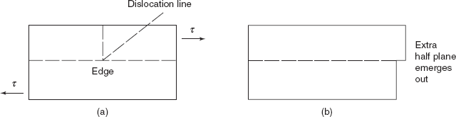
Figure 2.11 Edge dislocation

Figure 2.12 Screw dislocation
For an edge dislocation motion is parallel to shear stress. The net plastic deformation of both edge and screw dislocations is the same.
2.9 SURFACE IMPERFECTIONS
During solidification, the formation of new crystals in a polycrystalline material is random. Interaction of crystals between themselves inherits some imperfection on the inside surface. Grain boundaries are surface imperfections. Polycrystalline solids consist of several crystals of different sizes oriented randomly with respect to each other. They grow during the process of recrystallization, and the growth of crystals takes place by the addition of atoms. The crystals grow randomly (as shown in Figure 2.13) and in doing so impinge upon each other. When adjoining crystals impinge upon each other, some atoms are caught in between them. These atoms occupy position at the junction of adjoining crystals. Junction or the boundary is distorted and behaves as a non-crystalline material. This boundary region is a surface defect. Grain boundaries act as barrier to dislocation motion and restricting and hindering dislocation motion renders a material harder and stronger. A fine grained material is harder and stronger because fine grained material has greater total grain boundary area to impede dislocation motion.
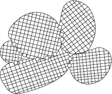
Figure 2.13 Randomly oriented grains
Sometimes during recrystallization twin boundaries are formed. The arrangement of atoms along twin boundary is such that one side of twin boundary is a mirror replica of the other side. Occurrence of twins is common in brass sheet or other metallic sheet.
In some cases, when crystal orientation is such that orientation angle between the two crystals is less than 10°, the boundary is called low angle tilt boundary.
2.10 VOLUME IMPERFECTIONS
Three-dimensional imperfections are found inside the solids. These may be due to one or more of the following reasons:
- Foreign particle inclusions.
- Regions of non-crystallinity.
- Pores.
- Dissimilar natured regions.
Virtually all crystalline materials contain some dislocations that were introduced during solidification and increased during plastic deformation or as a consequence of thermal stresses that result from rapid cooling. The number of dislocations or dislocation density in a material is expressed on the total dislocation length per unit volume.
Dislocation density as low as 103 mm/mm3 is found in a carefully solidified metal. For heavily deformed metals, the density may be as high as 109–1010 mm/mm3. Heat treatment of a deformed metal (say by annealing) can reduce the density to 105–106 mm/mm3.
2.11 SLIP SYSTEMS
Dislocations do not move with the same degree of ease on all crystallographic planes of atomic structure and in all crystallographic directions, but there is a preferred plane (slip plane) and a preferred direction (slip direction). For a particular crystal structure, the slip plane is that plane having the maximum atomic density (having maximum atomic planar density) and slip direction corresponds to the direction in this plane that is most closely packed with atoms.
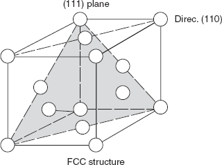
Figure 2.14 Slip plane
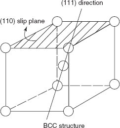
Figure 2.15 Slip plane and slip direction
FCC crystal: (as in Austenite) direction (111) plane
(Cu, Al, Ni, Ag, Au, etc.) [110] direction
Slip plane and slip direction for FCC crystal structure are shown in Figure 2.14.
BCC crystal: [110] slip plane
(Fe, W) [111] direction
Slip plane and slip direction for BCC crystal structure are shown in Figure 2.15.
HCP structure
(Cd, Mg, Ti)
Slip plane (0001)
Slip direction [11![]() 0]
0]
Slip plane and slip direction for HCP crystal structure are shown in Figure 2.16.
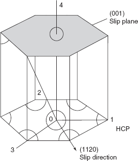
Figure 2.16 Slip plane and slip direction in HCP
2.12 MECHANICAL PROPERTIES
Mechanical behaviour of a material, i.e. its response or deformation to an applied external load in terms of strength, hardness, toughness, and ductility, is important for a structural or design engineer. Different types of loads as steady load, impact load, loads applied over long duration, cyclic loads, etc. are applied on standard specimen to study various mechanical properties.
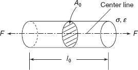
Figure 2.17 Gauge length of a standard sample
A simple tensile test is used to determine yield strength, ultimate strength, ductility, Young’s modulus of material. Figure 2.17 shows the gauge length of a standard sample, l0 area of cross-section is A0, subjected to tensile load F, then
engineering stress, ![]()
and
engineering strain,
If the graph between force and change in length is linear as shown in Figure 2.18(a), the slope of the curve between F versus dl gives Young’s modulus
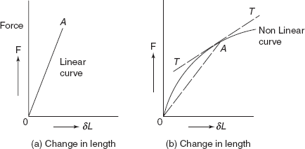
Figure 2.18 Force extension curves
As the bar elongates, there is increase in length but there is decrease in diameter of the bar. If the axial strain, i.e. δl/l, is positive, then lateral strain δD/D is negative. The ratio of lateral strain to longitudinal or axial strain is known as Poisson’s ratio.
For the non-linear behaviour, either tangent modulus or secant modulus is normally used. Figure 2.18(b) shows a non-linear graph between force and change in length.
At the point A, secant modulus
|
= slope of line OA = Esec |
tangent modulus, |
Etan = slope of tangent TT at A |
On atomic scale, Young’s modulus is defined as
where x is the distance between two atoms, and
x0 is interatomic distance for equilibrium.
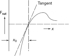
Figure 2.19 Net force vs interatomic distance graph
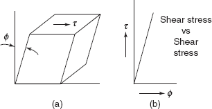
Figure 2.20 Shear stress and shear strain
Table 2.3 Elastic constants

Theoretical value of Young’s modulus on atomic scale is about 100 times the value of Young’s modulus of actual solid material (Figure 2.19).
If a rectangular block fixed at one face is subjected to shear stress τ on the opposite face, shear strain φ is developed. If variation of ϕ is linear with the variation of shear stress, τ, Figure 2.20.
Modulus of rigidity,
Elastic constants E, G, and v for engineering materials are given in Table 2.3.
2.12.1 Yield Strength
Yielding is characterized by initial departure from linearity of stress-strain curve. Deformation in any member after yielding has begun is permanent and many structures are designed only for the elastic deformation. Therefore, it is very important to know the yield point, where there is the onset of yielding. Figure 2.21 shows stress-strain curve for a ductile material, in which σ – ε curve has departed from linearity at point A. This point is known as yield point and the strength of the material at this point is known as yield strength. For some material, yield point is not clearly observed, where there is non-linear elastic region. The usual practice is to define the yield strength as a stress to produce some specified amount of strain, i.e. 0.002 or 0.2% strain as shown in Figure 2.22. A tangent is drawn at origin O on the non-linear σ – ε curve. Taking OB = 0.002 strain, a line BA is drawn parallel to tangent at O. Then stress at A (AB intersecting the stress-strain curve at A) is defined as 0.2%, Proof Stress.
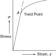
Figure 2.21 Stress-strain curve
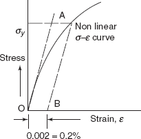
Figure 2.22 Proof stress
For some materials, elastic–plastic deformation is well defined and occurs abruptly at yield point. The material exhibits two yield points, i.e. upper and lower yield points. At the upper yield point, plastic deformation is initiated with an actual decrease in internal resistance of the material as in the case of mild steel, a medium carbon steel. This steel contains atmosphere of carbon and nitrogen atoms as impurities. Carbon and nitrogen atoms are smaller than iron atoms. During the plastic deformation, there is the movement of dislocations on slip planes and these dislocations glide over easily on carbon and nitrogen atoms and the resistance of the material is decreased but when these dislocations reach grain boundaries, the resistance of the material is increased because grain boundaries are harder than internal structure. As a result, there is increase in stress from lower yield point as shown in Figure 2.23. After upper yield point, continued deformation fluctuates slightly about some constant stress termed as lower yield point and subsequently rises with increasing strain, so the lower yield point is also known as point of strain hardening. At the maximum load, point D, a necking takes place in the material, and further extension takes places in the material in the vicinity of the neck. The material becomes plastically unstable, developing a neck. Dislocations in the material are responsible for neck formation. Stress at the maximum load is termed as ultimate tensile strength, i.e.
Specimen breaks making cup and cone type fracture, a typical behaviour of mild steel (Figure 2.24).
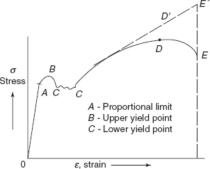
Figure 2.23 Stress-strain curve for mild steel
As the tensile deformation continues in the sample, the area of cross-section continuously decreases with deformation and true stress in the material is more than the engineering stress, in which original area of cross-section A0 is taken into account.
Area under the load-extension curve gives the energy absorbed by sample up to fracture-indicating toughness of the material.
If we assume constant volume during plastic deformation, then
|
At Lt = A0 L0 |
or |
P At Lt = P A0 L0 |
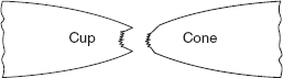
Figure 2.24 Cup-cone fracture
where At, Lt are true area and true length at same load P, A0, L0 are initial area of cross-section and length
So,
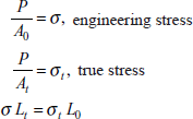
or true stress,
|
|
|
|
|
|
= |
σ(1 + ε), where ε is engineering strain. |
Similarly true strain is defined as the change in length at a particular stage divided by the length of sample up to that stage.
True strain, ![]()
Ductility of the material is defined by the percentage elongation in the sample up to fracture
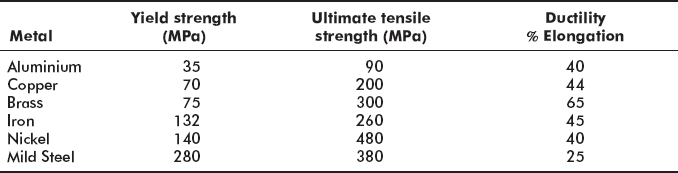
For common engineering materials, yield strength, ultimate tensile strength, and percentage elongation are given in Table 2.4.
Table 2.4 Mechanical properties
2.13 HARDNESS
Hardness of a material is defined as resistance of the material to (a) plastic deformation, (b) wear and tear, (c) scratch, (d) abrasion, etc. It is the most important property of a material because wear and tear or life of a material depend on its hardness. Generally, it is measured by localized plastic deformation caused by an indentor (of hardened steel or diamond) pressed on the surface of the material under a specified load.
A German Scientist employed the criterion of scratch and qualitatively decided on a Mohs scale of hardness ranging from 1 (for soft material) to 10 (for diamond).
But Brinell and Vicker’s have developed quantitative measurement of hardness by using a hardened steel ball indentor and a diamond indenter (of rhombus pyramid shape), respectively. Hardness is measured by taking compressive load in kgf and area of impression in mm2. Measurement and calculation of area of indented portion take some time. Rockwell has devised hardness measurement procedure by considering the depth of resulting indentation, and related the hardness to the depth of indentation, taking minimum time in hardness measurement.
2.13.1 Brinell Number
Indentors are made in various shapes, such as spheres, cones, and pyramids. The area over which the force acts increases with the depth of penetration. Figures 2.25(a) to (d) show the indentation produced on surfaces of sample by conical, square pyramid, knoop, and ball indentors. Around the indentation produced by a ball, the stress distribution is highly complex, because the material is forced outward from the region of indentation, triaxial stresses are produced in specimen which vary from the centre to the edge of the identation. Friction between ball and specimen produces hydrostatic stress.
In the case of pyramid indentors the sharp corners produce even more complex stress conditions.
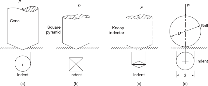
Figure 2.25 Various types of indentations
2.13.2 Pyramid Hardness
Diamond pieces are ground in the shape of square or rhombus pyramids.
Hardness number ![]()
where load |
P |
= |
λd2 where λ is a constant, and |
|
d |
= |
diagonal of square or rhombus indent. |
where β is another constant.
Hardness number, ![]()
Hardness number is λ/β independent of both the load and size of identation. It is easier to measure the diagonal of a pyramid indent due to sharp edges than to measure the diameter of a circular impression.
In the case of VPN (Vicker’s Pyramid Number) the angle between the opposite forces of the pyramid is 136°.
Surface of contact area between indentor and impression
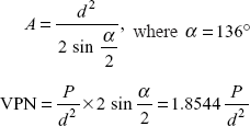
P in load in kg and diagonal in mm.
Knoop Indentor is developed especially to study the microhardness, i.e. the hardness of a microscopic area at selected site as in the individual metallic grain. Knoop hardness number is computed from the projected area of the impression.
Knoop Hardness ![]()
where P = Applied load in kg, and
d = Long diagonal of impression in mm.
Brinell Hardness Number: JA Brinell used hardened steel ball to determine the hardness of the metals
Area
where D = Diameter of the ball in mm, and
d = Diameter of the indentation in mm.
BHN is dependent on the load used. For this reason it is necessary to use the same load for all measurements with a given ball if a comparison of hardness of different metals is to be made.
2.13.3 Rockwell Hardness Test
This method is used to determine the hardness of a wide range of materials. Rockwell Hardness is measured by the use of a hardened steel ball (1.59 mm diameter) or a cone shaped diamond indentor (120° cone angle). In this test depth of impression is measured in place of diameter or diagonal of the impression. For the metallic specimen, three tests are used as:
Rock well A—For case hardened materials and thin metals such as razor blades.
Rock well B—For soft or medium hard metals as mild steel, brass, copper, etc.
Rock well C—For hard metals such as high speed steel, high carbon steel, tool steels, etc.
For Rockwell A and C, diamond indentor and for Rockwell B, steel ball indentor are used. A minor load of 10 kg is applied initially on the specimen through the indentor to overcome the thin oxide film on the metal. Then additional load of 50, 90, and 140 kg is applied on the indentor in the case of Rockwell A, B, or C, respectively.
Rockwell Hardness number
where |
H |
= |
a constant depending upon the scale, |
|
|
= |
130 for Rockwell B, |
|
|
= |
100 for Rockwell A and C, and |
|
t |
= |
depth of indent in mm and 0.002 mm corresponds to one unit of hardness number. |
2.13.4 Mechanism of Indent Formation
When the indentor is pressed onto the surface of a metal under a static compressive load, large amount of plastic deformation takes place under the indentor. The deformed material flows out in all directions. The region affected extends to a distance of about three times the radius of indentation, surface surrounding the impression bulges out slightly to account for the volume of the metal displaced under the indentor. In some cases ridging while in other cases sinking occur as shown in Figure 2.26. In the case of ridging type impression, the diameter of the indentation is greater than the true value, whereas with sinking type impression, the diameter of the impression is slightly less than the true value.
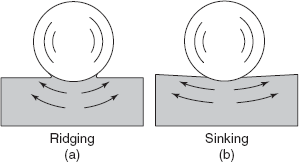
Figure 2.26 Indent formation
Plastic deformation during indentation is accompanied by large amount of transient creep which is time dependent. With the harder materials, the time required to reach the maximum deformation is nearly 15 seconds, such as for iron and steel. Soft materials like magnesium may require larger time, sometimes 2 minutes.
2.13.5 Rebound Hardness
Hardness is sometimes measured by dropping a hard object on the surface of a specimen and observing the height of its rebound. Usually a diamond point at the end of a small cylindrical piece is used to strike the surface. As it falls, its potential energy is converted into kinetic energy. A part of this kinetic energy is dissipated in producing plastic deformation of surface and rest is stored in recoverable elastic energy. The amount of strain energy absorbed in specimen depends upon its yield point, stiffness, and damping capacity. All the elastic strain energy is not recovered in the form of rebound of indentor due to the internal friction of the material. So, the rebound hardness measures a combination of hardness, stiffness, and damping capacity of the material.
In shore seleroscope test, a pointed hammer is allowed to fall from a height of 25.4 cm within a glass tube, which has a graduated scale inscribed on it. The standard hammer is approximately 6.35 mm in diameter, 1.9 cm long, and 2.4 gm in weight with a diamond tip of radius 0.25 mm. The scale is graduated in 140 divisions. A rebound of 100 is approximately equivalent to the hardness of a martensitic high carbon steel.
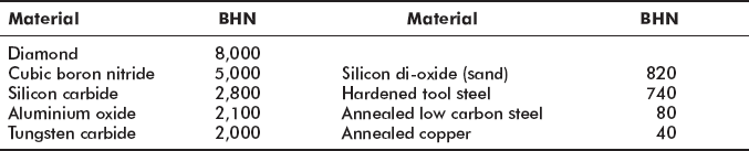
Diamond is the hardest material and in terms of kg/mm2, its hardness is extrapolated to 8000 BHN as shown in Table 2.5.
Table 2.5 Brinell hardness number of various materials
2.13.6 Superficial Hardness Test
In this test, the minor load is reduced from 10 to 3 kg and indentors are of diamond, ![]() dia ball and
dia ball and ![]() dia ball with major loads equal to 15, 30, and 45 kg applied as follows:
dia ball with major loads equal to 15, 30, and 45 kg applied as follows:
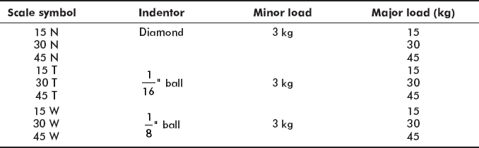
Example 2.1 60 HR 30 W indicates a superficial Rockwell Hardness of 60 on 30 W scale using ![]() ball indentor.
ball indentor.
An empirical relation exists between ultimate strength and BHN for most steels as follows:
2.14 FAILURE ANALYSIS
Failure of any engineering material is an undesirable event resulting in loss of human lives, materials, and disruption in services. In this chapter we will discuss about different types of fractures.
Simple fracture is the separation of a body into two or more pieces in response to imposed loads on body. The applied stress due to external loads may be tensile, compressive, shear, or torsional shear.
Let us first consider the effect of uniaxial tensile loads, due to which two fracture modes are possible, i.e. (a) ductile fracture with plastic deformation and (b) brittle fracture without any plastic deformation.
Figure 2.27(a) shows a highly ductile fracture, in which necking takes place to a point, as in the case of loading of a lead wire or a pure gold wire resulting in hundred percent reduction in area.
Figure 2.27(b) shows a moderately ductile fracture, after some necking as in the case of mild steel, under tensile load.
Figure 2.27(c) shows a brittle fracture, without any plastic deformation as in the case of grey cast iron under tensile load.
Ductility and brittleness are relative terms and ductility may be quantified in terms of (i) percentage elongation and (ii) percentage reduction in area. Ductility is a function of state of stress, strain rate, and temperature of the material.
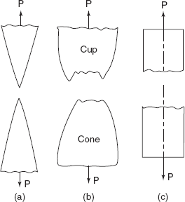
Figure 2.27 Different types of fractures
Any fracture process involves two stages, i.e. crack formation and crack propagation, in response to an imposed stress and the mode of fracture is highly dependent on the mechanism of crack propagation. Ductile fracture is characterized by extensive plastic deformation in the vicinity of an advancing crack and due to plastic deformation, the tip of the crack gets blunted resulting in stable crack and the fracture process proceeds slowly as the crack length is extended with an increase in applied stress. But in brittle fracture, cracks may spread extremely rapidly with very little accompanying deformation. Such cracks are unstable and crack propagation once started will continue spontaneously with any increase in applied stress.
Ductile fracture is always preferred over brittle fracture because of the following reasons:
- Brittle fracture occurs suddenly and catastrophically without any warning—a highly undesirable feature.
- In ductile fracture, the presence of plastic deformation gives warning and preventive measures can be taken.
- More strain energy is required to induce ductile fracture.
- Most metals and alloys are ductile.
- Ceramics are remarkably brittle.
- Polymers exhibit both types of fractures.
For common ductile materials, fracture is preceded by only a moderate amount of necking and fracture occurs in following stages:
- First of all necking begins.
- Small cavities or microvoids formed in the interior of cross-section.
- With continued deformation, microvoids enlarge and coalesce to form an elliptical crack.
- Rapid propagation of crack around the outer perimeter of the neck.
- Shear deformation of an approx 45° angle with the tensile stress axis.
- A cup and cone type fracture occurs as shown in Figure 2.27(b).
The central interior region of the fractured surface has an irregular and fibrous appearance, which is indicative of plastic deformation.
2.14.1 Brittle Fracture
In brittle fracture, the direction of a crack motion is very nearly perpendicular to the direction of applied tensile stress, resulting in a relatively flat surface of fracture. Any sign of gross plastic deformation is absent. Brittle fracture surfaces contain lines or ridges radiating from the origin of the crack in a form like pattern. Brittle fracture in amorphous materials such as ceramic glasses yields a shiny and smooth surface. For most brittle crystalline materials fracture is transgranular, i.e. fracture passes through grains. In some alloys, crack propagation is along grain boundaries and fracture is known as intergranular.
2.15 FRACTURE TOUGHNESS
Many ductile metals fracture abruptly with very little plastic deformation under some conditions. Following conditions are chosen for fracture impact test:
- Deformation at relatively low temperature.
- A high strain rate.
- A triaxial state of stress (which may be introduced by the presence of a notch).
Two standardized tests, i.e. (i) Charpy and (ii) Izod tests, are used to measure impact energy. In both tests a square cross-section bar with a V-notch of angle 45° and depth of 2 mm is taken as shown in Figures 2.28(a) and (b).
In the case of Izod impact test, specimen is positioned at the base as shown in Figure 2.28(a). A knife edge is mounted on the pendulum. When pendulum is released and fractures the specimen at the notch, which acts as a point of stress concentration for this high velocity impact blow, energy absorbed by the specimen is measured on a scale; this is known as impact energy. In the case of Charpy Impact Test, specimen is placed as a simply supported beam and pendulum strikes at the centre of the specimen.
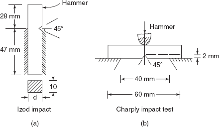
Figure 2.28 Impact test samples
2.15.1 Ductile to Brittle Transition
One of the primary features of Charpy or Izod tests is to determine whether or not a material experiences a ductile to brittle transition with decreasing temperature, if so then range of temperatures over which it occurs.
The ductile to brittle transition is related to the temperature dependence of the measured impact energy absorption. Figure 2.29 shows a curve for a steel. At higher temperature, the impact energy is relatively large in correlation with ductile mode of fracture. As the temperature is lowered, the impact energy drops suddenly over a relatively narrow temperature range, below which the energy has a constant but small value, and the mode of fracture is brittle.
Ductile fractured surface is fibrous and dull while a brittle fractured surface is granular and shiny.
For many alloys, there is a range of temperatures over which the ductile to brittle transition occurs. Structures constructed from alloys that exhibit ductile to brittle behaviour should be used only at room temperature to avoid brittle and catastrophic failure at the transition temperature (Figure 2.30).
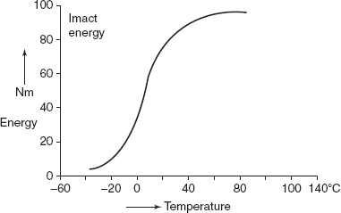
Figure 2.29 Ductile to brittle transition
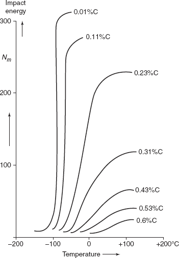
Figure 2.30 Influence of carbon content on Charpy V-notch energy vs Temperature
All metal alloys do not exhibit a ductile to brittle transition. Metals having an FCC crystal structure (including, aluminium, copper based alloys) remain ductile even at extremely low temperatures. But BCC and HCP alloys experience this transition. For these materials, the transition temperature is sensitive to both alloy composition and microstructure. For example, decreasing the average grain size of steels results in a lowering of the transition temperature. Hence, refining the grain size both strengthens and toughens steels. In contrast increasing the carbon content, while increasing the strength of steels also, raises the Charpy V-Notch Impact transition of steels.
Most ceramics and polymers also experience ductile to brittle transition, but for ceramic materials, transition occurs only at elevated temperatures ordinarily in excess of 1,000° C.
2.16 FATIGUE
Failure due to fatigue is characterized by cyclic stresses or fluctuating loads on structures like bridges, aircraft, turbine blades, springs, and machine components such as shafts, bearings. Failure due to cyclic stresses occurs at a stress level much lower than the tensile strength or yield strength under static load. About 90 per cent of failures in metallic components are due to fatigue fracture. The fracture due to fatigue is sudden and catastrophic and even a ductile material under fatigue loading behaves in a brittle manner. Fatigue fracture occurs in three stages, i.e.
- Nucleation of a fine crack on atomic scale,
- Propagation and growth of crack under continued cycles of stresses, and
- Sudden fracture, generally in a direction perpendicular to applied stress.
2.16.1 Cyclic Stresses
The applied stress may be axial (tension and compression), bending (completely reversed), or shear (torsional, twisting). In general, there are three different fluctuating stress versus time cycles possible (Figure 2.31), in which mean stress,
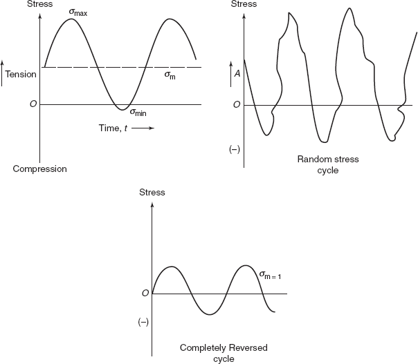
Figure 2.31 Stress cycles
Stress range, |
σr = σmax − σmin |
|
|
|
|
Random stress cycles are observed in aircraft wings during landing of the aeroplane. Completely reversed cycles produce maximum fracture effect; therefore in laboratory standard tests are performed on samples subjected to rotating bending as shown in Figures 2.32(a) and (b). In Figure 2.32(a) sample is loaded as a cantilever, producing bending moment WL at critical section. If d is the diameter of the sample at critical section then maximum bending stress
Cycle of stress as a particular point on the surface of the sample is also shown. Figure 2.32(b) shows a sample mounted as a simply supported beam and load W is applied through bearings on Section A and B, the bending moment on beam is constant between Sections A and B and is equal to Wa. Bending stress, σmax on surface
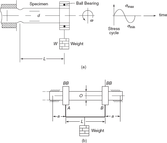
Figure 2.32 (a) Cantilever specimen (b) Pure bending sample
At a particular load, the specimens are allowed to rotate at frequency ω and number of the revolutions up to fracture of sample are noted on a revolution counter provided on the machine. For different stress levels, fatigue tests are performed and number of cycles required for fracture of sample is noted down. Then a graph between stress amplitude
and number of cycles required for fracture at each stress level is plotted as shown in Figure 2.33. Higher the magnitude of the stress, smaller is the number of cycles, the material is capable of sustaining before failure. For some ferrous (iron alloys) and titanium alloys S-N curve becomes horizontal at higher values of N, then limiting stress is called fatigue limit or endurance limit.
The fatigue limit represents the largest value of fluctuating stress that will not cause fracture for essentially an infinite number of cycles. For many steels fatigue limit ranges between 35% and 60% of the tensile strength.
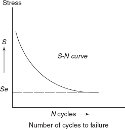
Figure 2.33 S-N curve
Most non-ferrous alloys (as of copper, aluminium, magnesium) do not have any fatigue limit. But the SN curve continues its downward trend at increasingly greater N-values. For such materials, fatigue strength at a particular value of N is defined as stress level at which failure will occur at some specified number of cycles.
There always exists a considerable scatter in fatigue data, i.e. variation in measured N values for a number of specimens tested at the same stress level, due to a number of factors such as fabrication and surface preparation, metallurgical variables, specimen alignment, etc. Several statistical techniques have been developed to specify fatigue life and fatigue limit in terms of probabilities. Generally these values are taken for 90% survivals. (At a particular stress, a number of specimens are tested, N is that value of number of cycles at which 90% of the total specimens tested have survived.)
Region of fractured surface that formed during stage II of crack propagation is characterized by two types of markings known as beach marks and striations. Beach marks are of macroscopic dimensions and striations are of microscopic size (Figure 2.34).
Final rapid failure may be either ductile or brittle. Generally ductile materials show plastic deformation at final fracture.
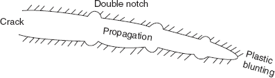
Figure 2.34 Crack propagation
2.16.2 Factors Affecting Fatigue Life
Fatigue behaviour of materials is highly sensitive to following variables:
(a) Mean stress, (b) Surface effects, and (c) Design details.
Dependence of fatigue life on stress amplitude is shown in Figure 2.35.
Increasing the mean stress level leads to a decrease in fatigue life (Figure 2.35).
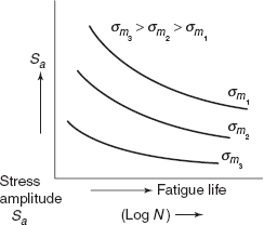
Figure 2.35 Stress amplitude fatique life
For many common loading conditions, the maximum stress within a component or a structure occurs at its surface. So, most cracks leading to fatigue failure originate at surface positions, specially at stress raiser sites. Fatigue life is sensitive to surface finish on component surface. Various surface treatments lead to improvement in fatigue life.
Design details of a component have significant influence on fatigue behaviour. Any notch (as keyway) or geometrical discontinuity (splines) acts as stress raisers. Sharper the discontinuity, more severe is the stress concentration. Fillet radius in a shaft is provided to reduce stress concentration at stepped section of shaft.
Fatigue behaviour is classified into two types, i.e.
- High loads—low cycle fatigue, producing not only elastic strain but plastic strain also, number of cycles is less than 103 – 105 cycles.
- Low loads—high cycle fatigue, wherein deformations are totally elastic, resulting in longer lives.
2.16.3 Crack Initiation and Propagation
The process of fatigue failure is characterized by three distinct stages: (i) crack initiation—a very fine crack forms at the same point of high stress concentration, (ii) crack propagation—during which this crack advances incrementally at each stress level, (iii) final fracture—which occurs very rapidly when the advancing crack has reached a critical size.
Fatigue life, |
Nf |
= |
Ni + Np |
|
|
= |
Number of cycles to crack initiation + number of cycles to crack propagation |
At low stress levels (high cycle fatigue) a large fraction of fatigue life is utilized in crack initiation. With increasing stress level, Ni decreases and cracks form more rapidly. Crack nucleation sites include surface scratches, sharp fillets, keyways, threads, dents, etc. In addition cyclic loading can produce microscopic discontinuities resulting from dislocation slip steps which may also act as stress raisers as crack initiation sites. Once a stable crack is initiated, it then propagates very slowly and in polycrystalline metals, along crystallographic planes of high shear stress—this is the first stage crack propagation. In the second propagation stage, crack propagation rate increases drastically and the direction of crack propagation roughly becomes perpendicular to applied tensile stress. During this stage of crack propagation, crack growth proceeds by a repetitive plastic blunting and sharpening process of the crack tip as shown in Figure 2.34.
2.16.4 Surface Treatments
During machining operations of components, due to tool action scratches are invariably introduced on surface of components. These surface scratches reduce the fatigue life. Polishing of surface enhances the fatigue life significantly.
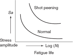
Figure 2.36 Stress amplitude fatique life
Another effective method of increasing fatigue performance is by imposing residual compressive stresses within a thin outer surface layer. Residual compressive stresses are introduced into ductile metals by shot peening, which causes localized plastic deformation in outer layer of surface. Small hard particles (shots) of diameters 0.1 to 1.0 mm are projected at high velocities on the surface to be treated. The resulting deformations induce compressive stresses to a depth of about one quarter and one half of shot diameter. Figure 2.36 shows improvement in fatigue performance due to shot peening.
2.16.5 Case Hardening
Case hardening enhances both surface hardness and fatigue life. In the case of carburising or nitriding process, a component is exposed to carbonaceous or nitrogenous atmosphere at an elevated temperature. A carbon- or nitrogen-rich outer surface layer (or case) is produced by atomic diffusion of carbon from the gaseous phase. Carbonaceous layer can be as thick as 1 mm and nitrogenous layer can be 0.2 mm thick.
2.16.6 Environmental Effects
If fatigue loading takes place in corrosive atmosphere, chemical attack during fatigue process is termed as corrosion fatigue and fatigue life is drastically reduced.
2.17 CREEP
ASTM defines creep as ‘time dependent strain under constant stress’. Many materials exposed to elevated temperatures are subjected to static mechanical stress, e.g. turbine rotors in jet engines and steam generators which experience centrifugal stresses and high pressure steam or gases. Deformation under such circumstances is termed as creep. Generally, the creep phenomenon is predominant in a material, when operating temperature is more than 0.4 Tm, where Tm is the melting temperature of the material. Amorphous polymers, plastics, and rubbers are especially sensitive to creep deformation.
A typical creep test consists of subjecting a specimen to a constant load or a constant stress while maintaining the temperature constant. Deformation (or strain) versus time is plotted as shown in Figure 2.37.
Most tests are of constant load type, which yield information of an engineering nature. But constant stress tests are employed to provide a better understanding of mechanism of creep. (In constant stress as extension continues, area of cross-section of sample continuously decreases, and a mechanism provides reduction in applied load, producing constant stress in sample).
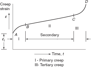
Figure 2.37 Constant load creep behaviour
Figure 2.37 indicates constant load creep behaviour showing:
- An instantaneous deformation or strain εi, mostly elastic (OA).
- A continuously decreasing creep rate—primary creep (AB) deformation becomes more and more difficult as the material is strained.
- Steady-state creep—rate is constant (BC), secondary creep—plot becomes linear.
This creep is of the longest duration. During secondary creep, creep rate remains constant due to balance between the process of thermal softening and strain hardening (due to plastic strain).
In the tertiary stage, strain rate accelerates and final fracture takes place resulting from microstructural changes and grain boundary separation, formation of internal cracks, cavities and voids. Also under tensile load a neck may form at some point in the sample. All these factors lead to a decrease in the effective cross-sectional area and increase in strain rate.
For metallic materials, most creep tests are performed in uniaxial tension. For brittle materials, uniaxial compression tests are performed, on specimens having l/d (aspect ratio) ratio equal to 2 to 4.
Important property from a creep test is creep rate, ![]() slope of secondary portion of creep curve.
slope of secondary portion of creep curve.
It is a useful parameter in engineering design, for long life operations of components in nuclear reactor power plant operating for several decades. Many short life creep tests are performed as on turbine blades in military aircraft, etc.
2.17.1 Stress and Temperature Effects
Both temperature and stress level influence the creep behaviour. At temperature considerably below 0.4 Tm (Tm is melting temperature), after initial instantaneous deformation, strain is virtually independent of time. With either increasing stress or increasing temperature, following will be noticed:
- Instantaneous strain at the time of stress application increases.
- Steady-state creep rate is increased.
- Rupture life time is diminished (Figure 2.38).

Figure 2.38 Creep curves at different temperatures
For some alloys and over relatively large stress ranges, non-linear behaviour is observed.
Steady-state creep rate
where K1 is a material constant, and
n is another material constant, neglecting the change in temperature.
if temperature influence is included, K2 is constant, Qa activation energy of creep.
2.17.2 Alloys for High Temperature Use
Many factors as melting temperature, elastic modulus, and grain size affect the creep behaviour of metals. In general, higher the melting temperature, greater the elastic modulus and larger the grain size, better is the resistance of metals to creep. Relative to grain size, smaller grains persist more grain boundary sliding, resulting in higher creep rate.
Stainless steels, refractory metals, superalloys are especially resistant to creep. The creep resistance of the Cobalt and Nickel superalloys is enhanced by solid solution alloying and also by the addition of a dispersed phase which is virtually insoluble in matrix.
2.18 STRESS RELAXATION
Bolts and fasteners required to hold two or more rigid plates in tight contact are frequently found to have relaxed considerably after long periods of time as a result of creep. This is called stress relaxation and defined as the time-dependent decrease in stress in a member which is constrained to a certain fixed deformation.
Let us consider that two plates are joined by a bolt and nut and εi = initial strain in bolt.
If this initial strain is maintained constant, the strain caused by creep is simply subtracted from it thereby reducing the elastic part of the total strain εi.
Elastic strain at any time,
The stress due to elastic strain εel i.e. εel × E goes on decreasing with time as shown in Figure 2.39.
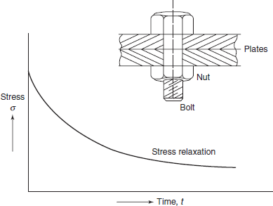
Figure 2.39 Stress relaxation curve
MULTIPLE CHOICE QUESTIONS
- A metallic specimen is loaded in tension beyond the yield point, then it is unloaded completely and then reloaded in tension again. After unloading and reloading, its yield point is
- slightly decreased
- slightly increased
- considerably decreased
- no effect on yield point
- The most important reason for Bauschinger’s effect in ductile materials is
- ductile materials weakness in shear
- compressive residual stress
- tensile residual stress
- None of these
- The notch angle in the Izod impact test specimen is
- 25°
- 30°
- 45°
- None of these
- Length of specimen fixed in vice in Izod Impact test is
- 40 mm
- 45 mm
- 47 mm
- 50 mm
- The angle between the opposite faces of the diamond pyramid in the case of Vicker’s Pyramid Hardness Test is
- 118°
- 120°
- 136°
- 140°
- Which indentor is used for Microhardness test
- Hardened Brinell ball
- Vickers Diamond Pyramid
- Conical shaped diamond
- Knoop Indentor
- The process which does not improve the fatigue strength of a material is
- The depth of penetration of the hardened steel ball in specimen is 0.140 mm. Rockwell Hardness of material is
- 60
- 65
- 70
- 75
- What is APF of an FCC crystal structure?
- 0.62
- 0.68
- 0.74
- 0.80
- What is the ratio of atomic radius of carbon atom to atomic radius of iron atom?
- 0.80
- 0.70
- 0.60
- 0.50
- Which of the following statements is incorrect?
- Point defects are thermodynamically stable
- Dislocations are not thermodynamically stable
- Screw dislocations are larger in number than edge dislocations in a crystal
- All of the above
- For FCC crystal, which direction is slip direction
- [110]
- [111]
- [1
 1]
1] - None of these
- What is Poisson’s ratio of Nickel?
- 0.33
- 0.31
- 0.30
- 0.28
- If ε is engineering strain and εt is true strain for a sample tested under tension, what is the relation between εt and ε?
- εt = 1n (1 + ε)
- εt = 1n (1 – ε)
- εt = 1n (ε)
- None of these
- Which of the following materials is remarkably brittle?
- Polymers
- Ceramics
- Bronzes
- None of these
- Which of the following materials fail in tension by making a necking to a point?
- Mild steel
- Wrought iron
- Lead
- Aluminium
- Which of the following statements is incorrect?
- Fatigue limit exists for most ferrous alloys
- For many steels fatigue limit ranges from 35% to 60% of tensile strength
- Increasing the mean stress level leads to increase in fatigue limit
- None of these
- Which of the following creep is of the longest duration?
- Primary creep
- Secondary creep
- Tertiary creep
- All the above have equal duration
Answers
1. (b) |
2. (b) |
3. (c) |
4. (c) |
5. (c) |
6. (d) |
7. (c) |
8. (a) |
9. (c) |
10. (c) |
11. (c) |
12. (a) |
13. (b) |
14. (a) |
15. (b) |
16. (c) |
17. (c) |
18. (b). |
|
|
PRACTICE PROBLEMS
2.1 Calculate APF of an HCP structure.
2.2 What is metallic bonding?
2.3 Explain edge dislocation. What is the difference between edge and screw dislocation?
2.4 What are surface imperfections?
2.5 For FCC and BCC structures mark slip planes and slip lines.
2.6 Explain the process of yielding in polycrystalline materials.
2.7 What is the reason of discontinuous yielding in mild steel?
2.8 Differentiate between:
- Elastic strain and Plastic strain
- Tangent modulus and Secant modulus
- Yield strength and 0.2% Proof stress.
2.9 Explain Bauschinger’s effect.
2.10 Draw stress-strain curve for cast iron in tension and in compression.
2.11 Mild steel and cast iron are tested up to destruction in tension. Compare their fractured surfaces.
2.12 Explain ductile to brittle transition of a material under impact loading.
2.13 Explain the purpose of a notch in a sample of impact testing.
2.14 Describe various types of indentors used in Hardness testing.
2.15 What is the mechanism of indentation when Brinell Ball is used for hardness measurement?
2.16 What are three stages of fatigue failure?
2.17 Explain how a submicroscopic crack is initiated during fatigue loading of a component?
2.18 What is the difference between fatigue strength and fatigue limit?
2.19 Explain the methods used for improving fatigue strength of a material.
2.20 Explain the temperature dependence of creep strain-time behaviour.