1
Elementary Elasticity
1.1 INTRODUCTION
An experimental stress analyst must have thorough understanding of stresses and strains developed in any structural member. Therefore, relationships between deformations, strains, and stresses developed in a body are derived in this chapter. Further generalized Hooke’s law, equilibrium equations and compatibility equations, and Airy’s stress functions for determining stresses at any point in a member subjected to known loads/stresses on its boundary form the text of this chapter. Plane stress state, plane strain state, and three-dimensional displacement field along with strain matrix are also discussed in the chapter.
1.2 STRESS TENSOR
All stresses acting on a cube of infinitesimally small dimensions, i.e. ∆x = ∆y = ∆z → 0 are identified by the diagram of stresses on a cube. The first subscript on normal stress σ or shear stress τ associates the stress with the plane of the stress, i.e. subscript defines the direction of the normal to the plane, and the second subscript identifies the direction of stress as
τxx = normal stress on yz plane in x-direction
τxy = shear stress on yz plane in y-direction
τxz = shear stress on yz plane in z-direction.
Similarly the stresses on xz plane and xy planes are identified as shown in Figure 1.1. Stress tensor τij can now be written as
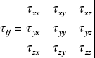
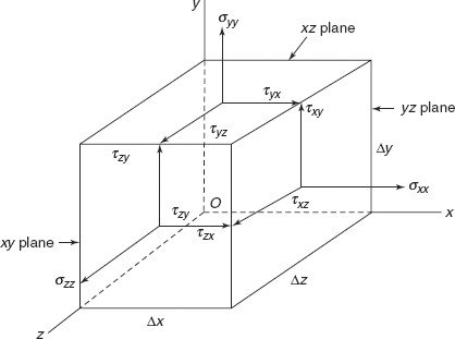
Figure 1.1 Stresses on a cube element
But, generally the normal stress is designated by σ.
So, τxx = σxx, τyy = σyy, τzz = σzz
Stress tensor can now be written as
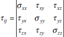
Stress tensor is symmetric, i.e. τij = τji
Complementary shear stresses are
Complementary shear stresses meet at diametrically opposite corners of an element to satisfy the equilibrium conditions.
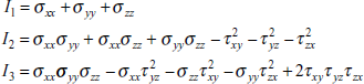
Stress invariants
1.3 STRESS AT A POINT
At a point of interest within a body, the magnitude and direction of resultant stress depend on the orientation of a plane passing through the point: An infinite number of planes can pass through the point of interest so, there are infinite number of resultant stress vectors. Yet the magnitude and direction of each of these resultant stress vectors can be specified in terms of the nine stress components as shown on three faces of elemental tetrahedron (Figure 1.2)
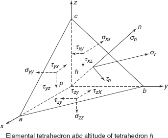
Figure 1.2 Stresses on elemental tetrahedron
Let us take the altitude of plane abc, h → 0 and neglecting body forces, three components of σr (resultant stress) in x-, y-, and z-direction can be written as
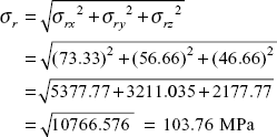
From these three Cartesian components, resultant stress, σr, can be determined as follows:
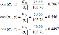
The three direction cosines which define the line of action of resultant stress σr are
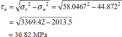
Normal stress σn and shear stress τn acting on the plane under consideration will be
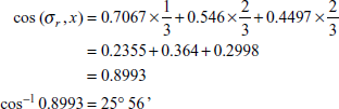
Angle between the resultant stress vector σr and normal to the plane σn can be determined by using
The normal stress σn also can be determined by considering projections of σrx, σry and σrz onto the normal to the plane under consideration; therefore
After the determination of normal stress σn, shear stress τn is obtained by
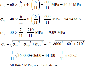
Example 1.1 At a point in a stressed body, the Cartesian components of stresses are σxx = 60 MPa, σyy = − 30 MPa, σzz = +30 MPa, τxy = 40 MPa, τyz = τzx = 0.
Determine normal and shear stresses on a plane whose outer normal has the direction cosines of
Solution: Let us say normal and shear stresses on plane are σn and τn, then resultant stress on plane is ![]()
For the problem, three components of σr are as follows:
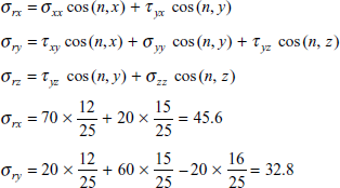
σrx = σxx cos(n, x) + τyx cos(n, y)
σry = τxy cos(n, x) + σyy cos(n, y)
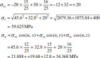
σrz = σzz cos(n, z) , because τyz = τyx = 0
Putting the values of σxx, σyy, σzz, τny, cos (n,x), cos (n, y),cos(n,z)
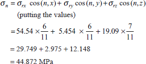
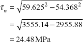
Shear stress,
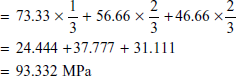
Example 1.2 At a point in a stressed body, the Cartesian components of stress are σxx = 70 MPa, σyy = 60 MPa, σzz = 50 MPa, τxy = 20 MPa, τyz = −20 MPa, τzx = 0.
Determine the normal and shear stresses on a plane whose outer normal has directions cosines
Solution:
Exercise 1.1 Determine the normal and shear stresses on a plane whose outer normal makes equal angles with the x, y, and z axes if the Cartesian components of stress at the point are
Ans. [σn = 120 MPa, τn = 43.20 MPa].
Exercise 1.2 At a point in a stressed body, the Cartesian components of stress are σxx = 40 MPa, σyy = 60 MPa, σzz = 20 MPa, τxy = 60 MPa, τyz = 50 MPa, τzx = 40 MPa, determine (a) normal and shear stresses on a plane whose outer normal has the directions cosines
(b) The angle between σr and outer normal n.
Ans. [σn = 117.77 MPa, τn = 58.547 MPa, angle 26°35’].
1.4 PLANE STRESS CONDITION
Under plane stress condition, stresses σxx, σyy, τxy are represented in one plane, i.e. central plane of a thin element in yx plane, as shown shaded in Figure 1.3
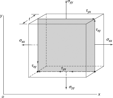
Figure 1.3 Plane stress state
In this case stresses σzz = τxz = τyz = 0.
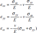
If E and v are Young’s modulus and Poisson’s ratio of the material, then strains are
Shear strain ![]()
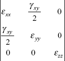
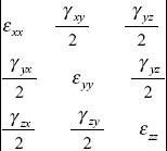
But shear strain γxy is equally divided about x and y axes both. Strain tensor for plane stress condition will be as follows:
For a particular set of three orthogonal planes, where shear stresses are zero and normal stresses on these planes are termed as principal stresses σ1, σ2, and σ3,
stress tensor will be 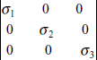
1.5 STRAIN TENSOR
Figure 1.4 shows a body of dimensions ∆ x and ∆y subjected to shear stresses τxy, τyx shear strain ![]() develops from y to x and from x to y.
develops from y to x and from x to y.
Total shear strain about xy axes is ![]()
where G is shear modulus.
This shear strain γxy is equally divided about both axes x and y. Strain tensor in a biaxial case will be

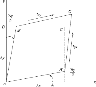
Figure 1.4 Shear stresses and shear strains on an element
Similarly strains ![]()
and ![]()
Three-dimensional strain tensor will be
In the plane stress case (σxx, σyy, τxy) the strains are
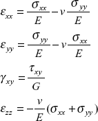
Strain tensor for a plane stress state is 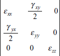
1.6 PLANE STRAIN CONDITION
For strain condition shown in Figure 1.5 the strain tensor is 
In this, strain
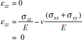
Therefore, σzz = v(σxx + σyy)
To satisfy the condition of plane strain
Moreover, γyz = γzx = 0
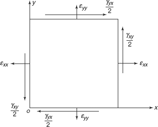
Figure 1.5 Plane strain state
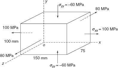
Figure 1.6 Example 1.3
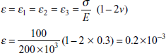
Example 1.3 A 100 mm cube of steel is subjected to a uniform pressure of 100 MPa acting on all faces. Determine the change in dimensions between parallel faces of cube if E = 200 GPa, v = 0.3.
Solution: σ = σ1 = σ2 = σ3 = 100 MPa, hydrostatic stress
Principal strains
Change in dimensions |
δ = δx = δy = δz = εa |
where |
a = side of cube |
Therefore |
= 100 × 0.4 × 10−3 |
|
= − 0.04 mm (because s is pressure) |
Exercise 1.3 A steel rectangular parallelopiped is subjected to stresses 100, − 60, + 80 MPa as shown in Figure 1.6. Dimension of the body are 150, 100, 75 mm in x-, y-, and z-direction. Determine change in dimensions, if E = 200 × 103 MPa, v = 0.3.
Ans. [+ 0.070 mm, − 0.057 mm, + 0.028 mm].
1.7 DEFORMATIONS
There are two types of strains resulting from deformation of a body, i.e. (a) linear or extensional strains and (b) shear strains, resulting in change of shape. Let us consider an element of dimensions ∆x, ∆y, with change in x- and y-direction as ∆x and ∆y as shown in Figure 1.7. A body of dimensions ∆x and ∆y, in x y plane, represented by ABCD, deforms to AB′C′D as shown in Figure 1.7(a).
Strain in x-direction, ![]()
Again it is deformed to A′B′CD as shown in Figure 1.7(b), strain in y-direction, ![]() .
.
Now the body in x-y plane is deformed to A′B′C′D, as shown in Figure 1.7(c).
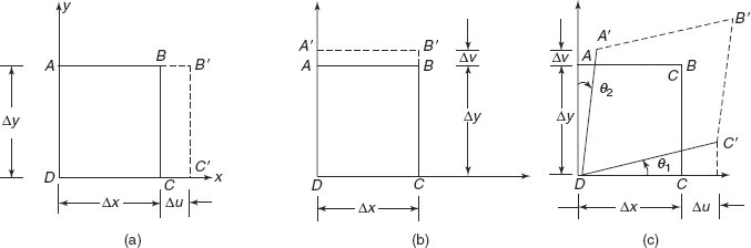
Figure 1.7 (a) Small element (b) Normal strain (c) Shear strains
Shear strain

Moreover, linear strains are ![]() on both side of coordinate axes
on both side of coordinate axes
In order to study the deformation, or change in shape, one has to consider a displacement field(s) for a point in a body subjected to deformation.
A point P is located at position vector op = r and displaced to position vector op′ = r′. The displacement vector S = r′ = r. The displacement vector (Figure 1.8) a function of x, y, z has components u, v, w in x-, y-, z-directions, such that
where S is a function of initial coordinates of point P.
function of x, y, and z.
These strains at point P are defined by
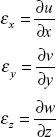
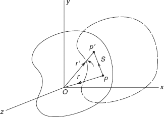
Figure 1.8 Displacement vectors
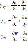
and shear strains are
In x-y plane, or in a two-dimensional case, strains are ![]()
Example 1.4 The displacement field for a given point of a body is 9 mm
at point P (1, −2, 3) determine displacement components in x-, y-, z-directions. What is the deformed position?
Solution: Displacement components are
Putting the values of initial co-ordinates (1,−2, 3) of point P components are
u = 1 + 2(−2) + 3 = 0.0
v = 3 × 1 + 4 × (−2)2 = 19 × 10−4
w = 2 × 13 + 6 × 3 = 20 × 10−4
x′ = x + u = 1 − 0 = 1
y′ = y + v = −2 + 19 × 10−4 = −1.9981
z′ = z + w = 3 + 20 × 10−4 = 3.002
Example 1.5 The displacement field for a body is given by
write down the strain components and strain matrix at point (2,1,2).
Solution: Displacement components are
Putting the values of initial co-ordinates (2, 1, 2)
strain matrix 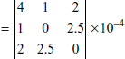
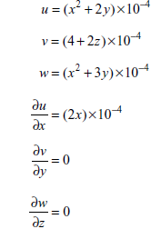
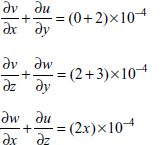
Example 1.6 Displacement field is S = [(x2 + y2 + 2)i + (3x + 4y2)j] × 10−4 what is strain field at point (1, 2)?
Solution: Displacement components are
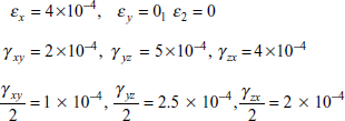
Strain components
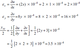
Strain tensor ![]()
Exercise 1.4 The displacement field for a body is given by S = [(x2 + 2y)i + (3y + z)j + (x2 + z)k] × 10−3 what is the deformed position of point originally at (3, 1, −2)? Write down strain matrix.
Ans. [3.011, 1.001, −1.993], 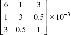 .
.
Exercise 1.5 Displacement field is
where k is a very small quantity.
What are strains at (1, −2) point?
Ans. [4k, −8k, +2k].
1.8 GENERALIZED HOOKE’S LAW
For a simple prismatic bar subjected to axial stress σxx and axial strain εxx (Figure 1.9), Hooke’s law states that stress ∝ strain
|
σxx ∝ εxx |
|
|
σxx = E εxx |
(1.1) |
where E is proportionality constant and E is Young’s modulus of elasticity of the material.
But for an elastic body subjected to six stress components σxx, σyy, σzz, τyx, τyz, τzx and six strain components, i.e. εxx, εyy, εzz, γxy, γyz, γzx, the generalized Hooke’s law can be expressed as
σxx |
= |
A11 εxx + A12 εyy + A13 εzz + A14 γxy + A15 γyz + A16 γzx |
|
σyy |
= |
A21 εxx + A22 εyy + A23 εzz + A24 γxy + A25 γyz + A26 γzx |
|
σzz |
= |
A31 εxx + A32 εyy + A33 εzz + A34 γxy + A35 γyz + A36 γzx |
(1.2) |
τxy |
= |
A41 εxx + A42 εyy + A43 εzz + A44 γxy + A45 γyz + A46 γzx |
|
τyz |
= |
A51 εxx + A52 εyy + A53 εzz + A54 γxy + A55 γyz + A56 γzx |
|
τxz |
= |
A61 εxx + A62 εyy + A63 εzz + A64 γxy + A65 γyz + A66 γzx |
|
where A11, A12, …, A65, A66 are 36 elastic constants for a given material.
For homogeneous linearly elastic material, above noted six equations are known as generalized Hooke’s law. Similarly, strains can be expressed in terms of stresses as follows:
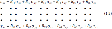
For a fully anisotropic material there are 21 constants ![]() in generalized Hooke’s law and for orthotropic materials there are nine constants in Hooke’s law.
in generalized Hooke’s law and for orthotropic materials there are nine constants in Hooke’s law.
Say for an isotropic material having the same elastic properties in all directions and material as such has no directional property, there are three principal stresses σ1, σ2, σ3 and three principal strains ε1, ε2 and ε3, then Hooke’s law can be written as
where A, B, and C are elastic constants.
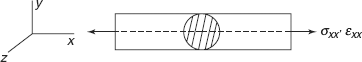
Figure 1.9 Simple bar subjected to axial stress and axial strain
In the above equation ε1 is the longitudinal strain along σ1 but ε2 and ε2 are lateral strains so, constants B = C, therefore
|
σ1 |
= |
A ε1 + B ε2 + C ε3 |
|
|
= |
A ε1 + B ε1 − B ε1 + B ε2 + B ε3 |
|
|
= |
(A − B)ε1 + B(ε1 + ε2 + ε3) |
where ε1 + ε2 + ε3 = ∆, a cubical dilatation = first invariant of strain
Let us denote (A − B) by 2 μ and B by λ, then
|
σ1 = λ Δ + 2με1 |
(1.5) |
Similarly |
σ2 = λ Δ + 2με2 |
(1.6) |
|
σ3 = λ Δ + 2με3 |
(1.7) |
λ and μ are called Lame’s coefficients.
From Eqs (1.5), (1.6), and Eqs (1.7)
|
σ1 + σ2 + σ3 |
= |
3λ Δ + 2μ(ε1 + ε2 + ε3) |
|
|
= |
3λ Δ + 2μ Δ |
|
|
= |
(3λ + 2μ) Δ |
Principal stress
Solving Eq (1.9) for ε1, we get
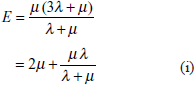
From elementary strength of materials
Therefore, Young’s modulus ![]()
Poisson’s ratio, ![]()
Example 1.7 For steel Young’s modulus E = 208000 MPa and Poisson’s ratio, v = 0.3. Find Lame’s coefficients λ and μ.
Solution:
Taking Eq. (i)
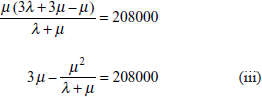
From Eq. (ii)
or |
λ = 0.6 λ + 0.6 μ |
|
|
λ = 1.5 μ |
(iv) |
Putting this value in Eq. (iii)
Lame’s coefficient, |
μ = 80000 N/mm2 |
Coefficient, |
λ = 1.5 μ = 120000 N/mm2 |
Exercise 1.6 For a concrete block E = 27.5 × 10³ MPa and Poisson’s ratio is 0.2. Determine Lame’s coefficients λ and μ.
Ans. [7639 N/mm2, 11458 N/mm2].
1.9 ELASTIC CONSTANTS K AND G
From the previous article 1.8, we know that
Putting the value of ![]() from Eqs (1.12) in Eqs (1.11), we get
from Eqs (1.12) in Eqs (1.11), we get
From the elementary strength of material we know that
Therefore Lame’s coefficient μ = G, shear modulus. From Eqs (1.8) of previous article. If σ1 = σ2 = σ3 = p, hydrostatic stress or volumetric stress
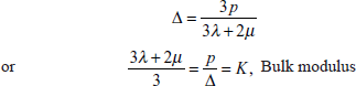
Therefore, Bulk modulus, ![]()
Shear modulus, G = μ, Lame’s coefficient.
Example 1.8 For aluminium E = 67000 MPa, Poisson’s ratio, v = 0.33. Determine Bulk modulus and shear modulus of aluminium.
Solution:
or
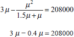
From Eq. (ii)
Poisson’s ratio
or
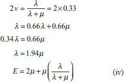
Putting the value of λ in terms of μ in Eq. (iv)
|
E |
= |
2μ + μ × 0.66 = 2.66μ |
|
|
|
|
|
|
|
|
= |
Lame’s coefficient |
|
|
|
= |
Shear modulus |
|
|
G |
= |
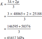
25188 MPa |
(v) |
|
λ |
= |
1.94μ = 1.94 × 25188 = 48865 MPa |
|
Bulk modulus,
Exercise 1.7 For steel E = 200000 MPa and Poisson’s ratio is 0.295. Determine Lame’s coefficients and Bulk modulus K.
Ans. [λ = 111120 MPa, μ = 77220 MPa, K = 162600 MPa].
1.10 EQUILIBRIUM EQUATIONS
Consider a small infinitesimal element of a body of dimensions ∆x, ∆y and thickness t = 1 subjected to stresses varying over distances ∆x and ∆y as shown in Figure 1.10. X and Y are body forces per unit volume in x- and y-directions.
Taking the summation of forces in x-direction
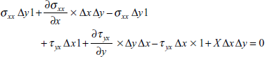
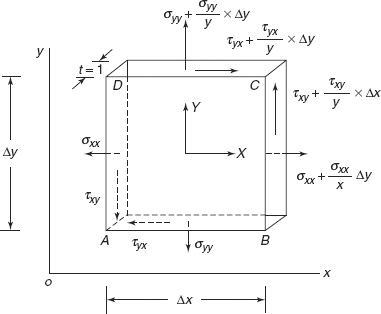
Figure 1.10 A small infinitesimal element in equilibrium
or
Simplifying further
Taking the summation of forces in y-directions
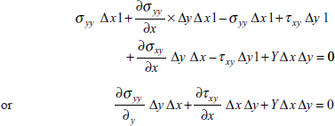
Simplifying further
In three-dimensional case equilibrium equations can be written as
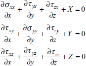
where X, Y, Z are body forces per unit volume.
In these equations, mechanical properties have not been used. So, these equations are applicable whether a material is elastic, plastic or viscoelastic.
In a two-dimensional case, equilibrium equations are
|
|
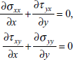
We may permanently satisfy these equations by expressing stresses in terms of a function ϕ, called Airy’s stress function, as follows:
In a plane stress case a body subjected to stresses σxx, σyy, τxy, the strains are
Shear strain,
Strain compatibility equations are
Substituting the values of εxx, εyy, γxy from Eqs (1.15), (1.16), and Eq (1.18) in Eq (1.19), we will get
Putting the value of ![]() in Eq (1.20), we get
in Eq (1.20), we get
Simplifying further the equation becomes
or Δ ϕ = 0 (1.21)
Airy’s stress function ϕ chosen for any problem must satisfy the above Biharmonic equation.
Example 1.9 Following strains are given
|
εxx |
= |
6 + x2 + y2 + x4 + y4 |
|
εyy |
= |
4 + 3x2 + 3y2 + x4 + y4 |
|
γxy |
= |
5 + 4xy(x2 + y4 + 2) |
|
|
= |
5 + 4x3y + 4xy3 + 8xy |
Determine whether the above strain field is possible. If it is possible determine displacement components u and v, assuming u = v = 0 at origin.
Solution: Strain compatibility condition is
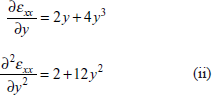
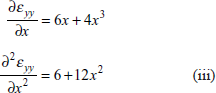
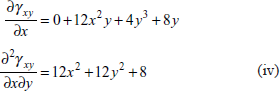
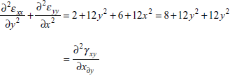
Strain field is possible.
Now
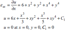
Displacement component
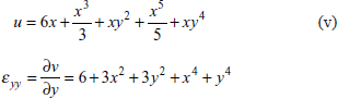
Integrating
but v = 0 at x = 0, y = 0, constant C2 = 0
so, ![]()
Exercise 1.8 Given the following system of strains
|
εxx |
= |
8 + x2 + 2y2 |
|
εyy |
= |
6 + 3x2 + y2 |
|
γxy |
= |
10xy |
Determine whether the above strain field is possible. If possible determine displacement components u and v if u = 0, v = 0 at origin.
Ans. [strain field is possible]
1.11 SECOND DEGREE POLYNOMIAL
Let us consider an Airy’s stress function
∇4 ϕ = 0 satisfies the compatibility condition
|
|
|
|
Shear stress, ![]() (negative, tends to rotate the body in anticlockwise direction). This represents a plane stress condition as shown in Figure 1.11.
(negative, tends to rotate the body in anticlockwise direction). This represents a plane stress condition as shown in Figure 1.11.
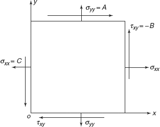
Figure 1.11 Plane stress condition
Example 1.10 Airy’s stress function ϕ = 40 x2−30 xy + 60 y2 satisfies the compatibility condition ∇4 ϕ = 0. Determine stresses σxx, σyy and τxy, Show graphically the stress distribution. Stresses are in MPa.
Solution: ϕ = 40x2 − 30 xy + 60y2
|
|
|
|
|
|
|
|
|
|
|
|
|
|
|
Note that shear stress, τxy is + ve, i.e. tending to rotate the body in a clockwise direction. Figure 1.12 shows the stress distribution which is a plane stress state. τyx are shear stresses complementary to τxy.
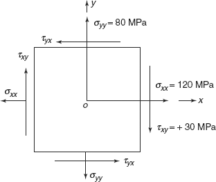
Figure 1.12 Stresses on element
Exercise 1.9 An Airy’s stress function ϕ = 50 x2 − 40 xy + 80 y2 satisfies the compatibility condition ∇4 ϕ = 0. Determine normal and shear stresses and state the type of state of stress.
Ans. [σxx = 160 MPa, σyy = 100 MPa, τxy = +40 MPa, a plane stress condition].
1.12 A BEAM SUBJECTED TO PURE BENDING
For a beam of depth d subjected to pure bending moment M and no shear force, as shown in Figure 1.13. Airy’s stress function can be a third degree polynomial
∇4 ϕ = 0, for this function
Taking B = 0 as stress σxx is independent of x,
y varies from − ![]() to +
to + ![]() as shown in Figure 1.14.
as shown in Figure 1.14.
Maxm. σxx in tension
where

Maxm.σxx in compression
where M = bending moment M, and
I = second moment of area (of cross section of beam) about neutral plane.
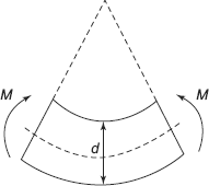
Figure 1.13 Beam subjected to pure bending
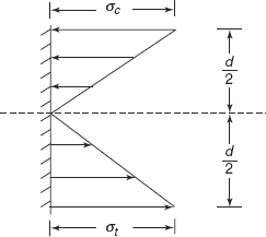
Figure 1.14 Stress distributions
Now ![]()
but σyy = 0, so constant C = D = 0
Shear stress ![]()
but |
= By + Cx |
|
τxy = 0, |
also because it is a case of pure bending.
So, constants B = C = 0
Finally Airy’s stress function is ![]() .
.
Example 1.11 A bar of circular section of diameter 30 mm is subjected to a pure bending moment of 3 × 10⁵ Nmm. What is the maximum bending stress developed in beam? What is Airy’s stress function for this case.
Solution: Moment of inertia of beam,
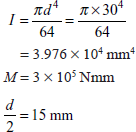
Bending stress
Airy’s stress function for this case

where
Airy’s stress function ϕ = 1.257 y3
where y varies from − 15 to + 15 mm.
Exercise 1.10 For a beam of rectangular section B = 20 mm, D = 30 mm, Airy’s stress function ϕ = 1.6 y3.
Determine the magnitude of constant BM acting on beam section.
Ans. [432 Nm].
Problem 1.1 A beam of rectangular section is subjected to shear force F = 1 kN and bending moment = −1 × 10⁶ Nmm. Section of beam is B = 20 mm, D = 60 mm. Write down stress tensor for an element located at 15 mm below the top surface (see Figure 1.15).
Figure 1.15 Problem 1.1
Solution:
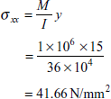
M = −1 × 10⁶ Nmm (producing convexity)
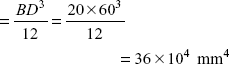
I = second moment of area about neutral plane
y = 15 mm from neutral layer.
Bending stress,
To determine shear stress at y = 15 mm from neutral layer
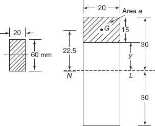
Figure 1.16 Problem 1.1
where area a = 15 × 20 = 300 mm2 = area of section above the layer under consideration,
ӯ |
= |
225.,mm distance of CG of area a from neutral layer, |
b |
= |
breadth = 20 mm, |
I |
= |
36 × 104 mm4, |
F |
= |
1 kN = 1000 N, |
|
|
|
|
= |
0.9375 N/mm2. |
Stress tensor for this state of stress, at a layer 15 mm below top surface
Problem 1.2 At a point in a stressed body the Cartesian components of stress are σxx = 80 MPa, σyy = 50 MPa, σzz = 30 MPa, τxy = 30 MPa, τyz = 20 MPa, and τzx = 40 MPa, determine (a) normal and shear stresses on a plane whose normal has the direction cosines
(b) angle between resultant stress and outer normal n.
Solution: Components of resultant stress σr are
Substituting the values as above
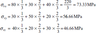
Normal stress, σn = σrx × cos(n, x) + σry cos(n, y) + σrz cos(n, z)
Shear stress,

Angle between resultant stress vector σr and normal to the plane n is given by
where
So,
Problem 1.3 A cantilever beam of rectangular section B × D and of length L carries a concentrated load W at free end Figure 1.17. Consider a section at a distance x from fixed end and a layer at a distance y from neutral layer zz; derive expression for Airy’s stress functions
if |
B = 40 mm, D = 60 mm |
|
W = 1 kN, x = 2 m, L = 5 m |
Write stress tensor for the layer bc, if y = 20 mm
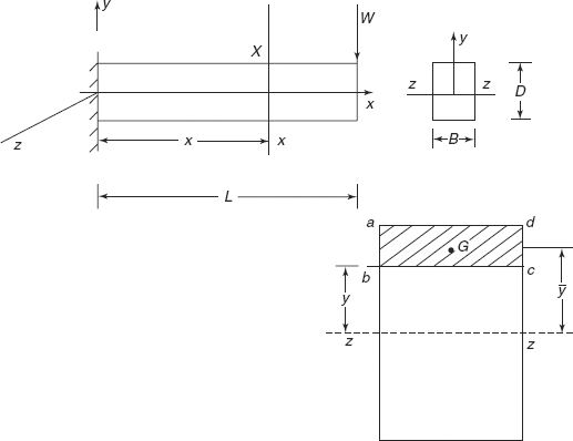
Figure 1.17 Problem 1.3
Solution: Stresses
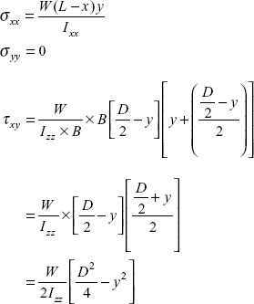
Let us assume Airy’s stress function ϕ = C1y3 + C2 xy3 + C3 xy.
- For
 τxy = 0, σyy = 0
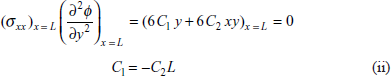
 - For x = 0, σxx = 0
- Everywhere
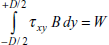 , shear force is constant
Applying these boundary conditions
So, ![]()
or
Moreover

or
Putting the value of ![]() C2D2 in Eq. (iii)
C2D2 in Eq. (iii)
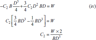
Then
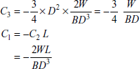
Finally, Airy’s stress function is
At the layer where x = 2 m = 2000 mm, L = 5000 mm

Strees tensor ![]()
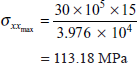
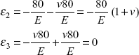
Problem 1.4 A solid circular shaft of steel is transmitting 100 hp at 200 rpm. Determine shaft diameter if the maximum shear stress in shaft is not to exceed 80 MPa. Write down stress tensor for the surface of the shaft. Show that surface of the shaft is under both plane stress and plane strain conditions E = 200 × 103 N/mm2, v = 0.3.
Solution: HP transmitted = 100
RPM, N = 200
angular speed, ![]()
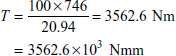
Torque transmitted, = 20.94 rad/s
Torque transmitted,
Maxm. Shear strees,
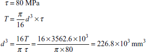
Shaft diameter d = 60.87 mm
On the surface of the shaft, τ = ± 80 MPa
Principal stresses on the surface of the shaft are
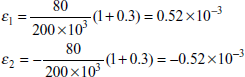
Principal strains,
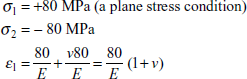
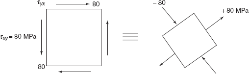
Figure 1.18 Problem 1.4
Since ε3 = 0, this a plane strain condition.
Strain are
Stress tensor
Stress tensor
MULTIPLE CHOICE QUESTIONS
- Principal stresses at a point are 120, −40,−20 MPa. What is maximum shear stress at the point?
- 50 MPa
- 70 MPa
- 80 MPa
- None of these
- A bar is subjected to axial load such that its length l is increased by 0.001 l. If Poisson’s ratio is 0.3, what is change in its diameter d?
- −3 × 10⁻⁴ d
- +3 × 10⁻³ d
- +3 × 10⁻⁴ d
- None of these
- Lame’s coefficient for a material are λ and m. What is Poisson’s ratio?


- None of these
- Ratio of volumetric stress/volumetric strain is known as
- Shear modulus
- Bulk modulus
- Young’s modulus
- None of these
- Airy’s stress function is ϕ = 50x2-40xy+80y2, what is normal stress syy
- 100 MPa
- 40 MPa
- +160 MPa
- 80 MPa
- A rectangular section beam of breadth b, depth d is subjected to shear force F. At what depth y from top surface transverse shear stress is maximum
- y = 0


- A shaft is subjected to pure twisting moment M. Surface of the shaft represents
- Plane strain condition
- Plane stress condition
- Both plane stress and plane strain conditions
- Neither plane stress nor plane strain condition
- A thin metallic sheet is subjected to inplane shear stress, what is the state of stress of thin sheet ?
- a plane strain state
- a plane stress state
- a hydrostatic state of stress
- None of these
Answers
1. (c) |
2. (a) |
3. (b) |
4. (b) |
5. (a) |
6. (d) |
7. (c) |
8. (b). |
|
|
EXERCISE
1.1 Consider a beam of rectangular section B = 25 mm, D = 60 mm subjected to a bending moment + 1.5 × 10⁶ Nmm. Write down (i) the stress tensor for an element located at top surface and (ii) the stress tensor for an element located in a plane 15 mm below the top surface.
Ans. ![]()
1.2 For a material, Lame’s coefficients are
λ = 1.2 × 10⁵ MPa, μ = 0.8 × 10⁵ MPa. Determine E, v, and G for the material.
Ans. [E = 208000 MPa, v = 0.3, G = 80,000 MPa].
1.3 A cantilever of rectangular section B × D is of length L as shown in Figure 1.19. Write down stress tensor to determine state of stress at section XX at a distance of x from free end and at layer at distance of y from neutral layer.
Ans.
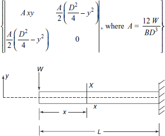
Figure 1.19 Exercise 1.3
1.4 A cylindrical bar of length L, area of cross section A is fixed at top end. Write down Air’s stress function for stress due to self weight in bar, if w is the weight density of the bar (see Figure 1.20).
Ans. ![]()
1.5 Consider the displacement field S = (y2 i + 3yx j) × 10−2. Find whether strain field is compatible. If yes find strain components εx, εy, ![]() at point (1, −1).
at point (1, −1).
Ans. 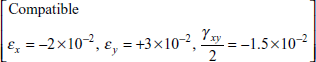
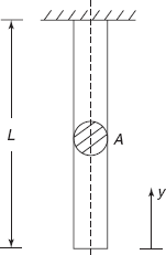
Figure 1.20 Exercise 1.4