
13
Experiments in Material Testing and Experimental Stress Analysis
13.1 INTRODUCTION
At the undergraduate level, in the course of strength of materials/mechanics of solids, many tests are conducted such as hardness test, impact test, tensile test, compression test, etc. but at this stage we will discuss mechanical tests such an true-stress strain curve for a ductile material in tension, buckling test on column, creep test on a wire, fatigue test on rotating–bending specimen, and tests on experimental stress analysis techniques using photoelastic, strain gauges, and brittle coating techniques, etc.
Most important mechanical test is a simple tensile test on sample because this test provides a lot of vital information about mechanical behaviour of a metal, useful for designing a machine component. Ductility of a metal is noted by its percentage elongation, degree of cold working is obtained by its percentage reduction in area, strengths at yield point and at ultimate load are obtained.
For industry, fatigue test, creep test, and shear centre test for unsymmetrical bending are important and will be discussed in this chapter. Calibration of a photoelastic model for stress fringe value will also be described. Use of strain gauges on transducers, for the measurement of force, torque, and bending moment, will also be discussed and calibration constants for transducers will be derived.
13.2 TO PLOT A GRAPH BETWEEN ACTUAL STRESS AND ACTUAL STRAIN FOR A SAMPLE UNDER TENSION USING UTM
Figure 13.1 shows various types of tensile test samples which can be tested on a universal testing machine. Figure 13.1(a) shows a sample with threaded portion at the ends and such a sample is screwed in grips provided in the fixed and movable cross heads of a universal testing machine. Figure 13.1(b) shows a sample with plane circular ends, and wedge grips in machine are required for firm gripping of this sample. Figure 13.1(c) shows a sample with collars at the ends. Special grips are provided for such a sample. For the measurement of extension in the beginning, an extensometer can be connected over a gauge length of 50 mm. There are various capacities of any u.t.m. Depending upon the requirement, the capacity of the machine is selected and the strain rate is adjusted so as to have minimum strain rate, and the specimen is slowly and gradually extended. Once the specimen is firmly gripped, machine is put on and the readings of load and extension are simultaneously recorded. Now-a-days, an automatic graph is obtained between load and extension on the testing machine.
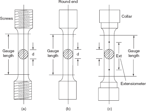
Figure 13.1 Tensile test specimens
While performing the tension test on a mild steel specimen, the load increment should be carefully checked, because at the upper yield point there is a slight reduction in load and then the load again continuously increases and at a particular instant the test piece breaks at the neck formed in sample (in case of a ductile material). From the automatic graph or graph plotted between load and extension, various mechanical properties are determined.
To note down the percentage reduction in area, the two broken pieces of sample are joined together and the diameter at the neck is measured.
Say |
D = diameter of the sample |
|
d = diameter at the neck (after fracture) |
To determine the value of percentage elongation join the two broken pieces and measure the changed gauge length.
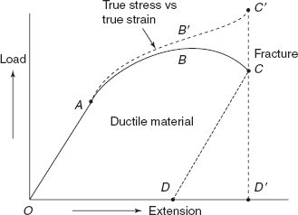
Figure 13.2 Load extension diagram in tension
Say |
L = initial gauge length |
|
L′ = final gauge length |
It is necessary to note down the change in gauge length from the broken pieces because once the fracture occurs, the load is removed from the specimen and the elastic part of the deformation is recovered immediately as shown in Figure 13.2 by the portion D’D. Line CD is parallel to the straight line portion OA of the graph.
After the yield point, once the plastic deformation has started, the cross sectional area of the specimen starts decreasing at a faster rate and the actual stress at any instant (in the plastic stage) is much more than the nominal stress (calculated on the basis of original area of cross section)
Engineering stress, ![]()
original length = L
original area of cross section, ![]()
From the graph of load and extension curve, a table can be made for the observation of load P and extension dL, the ratio of dL/L gives engineering strain ε and ratio of P/A (original area of cross section) gives the value of engineering stress σ.
Table 13.1 shows the values of σ, ε, σt, and ε, for different values of P and dL.
Table 13.1 True stress and true strain
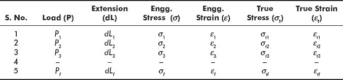
Figure 13.2 shows graphs between engineering stress and engineering strain O A B C and between true stress and true strain, represented by curve O A B′ C′.
Precautions:
- Grip the specimen firmly in grips.
- Adjust suitable capacity of the machine and strain rate.
- Record the readings of load and extension simultaneously.
- Continuously watch the movement of the pointer on the load scale so as to clearly get upper and lower yield points (in the case of mild steel).
- Once the neck is formed in the sample, decrease the strain rate.
- In the beginning adjust the pointer at the zero of the load scale.
13.3 BUCKLING TEST ON COLUMNS USING U.T.M.
The aim of this experiment is to determine Rankine’s constants σc and a in the Rankine’s buckling load,
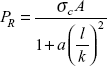
where A is the area of cross-section of the column, l is the length of the column, and k is the minimum radius of gyration of the section of the column.
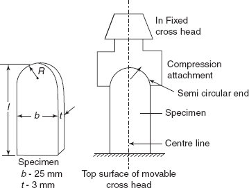
Figure 13.3 Specimen under buckling test
The shape of the specimen is shown in Figure 13.3. The specimen is of rectangular section b × t with a flat end and a semicircular end. The length of the specimen (or column) is taken from bottom to the top edge. Several samples of lengths 50, 60, 70, 80, 90, 100 mm are made from mild steel, the most common structural steel. The specimen is placed in a vertical position on the top of the movable cross head and compression block with a hemispherical cavity is fitted in the bottom of the fixed cross head of the u.t.m. The strain rate is adjusted and machine is put on. Once the clearance between specimen and hemispherical cavity is filled, load starts acting on the column. Continuously watch the movement of the pointer on the load scale. At a particular instant, column buckles and load is suddenly reduced. Note down the maximum load at this stage of buckling. For various samples of different lengths note down the buckling loads as shown in Table 13.2.
Plot a graph between PR and l as shows in Figure 13.4. Plot the graph through the mean positions of observations and take two points on graph as shown. Note down P1, l1 and P2, l2 from the graph and calculate the Rankine’s constants σc and a.
Precautions:
- Lower end of the sample must be flat and perpendicular to the axis of the sample.
- Upper end of the sample must be semi-circular fitting into the cavity of compression attachment.
- Place the sample in the vertical position, on the movable head of u.t.m.
- Apply the load slowly and gradually.
- Continuously watch the pointer on load scale so as to note down the exact buckling load.
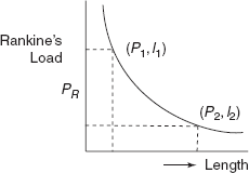
Figure 13.4 Rankine’s load vs length graph
Table 13.2 Readings of sample length and buckling load
| Length of sample, l | Bucking load PR in kN |
|---|---|
50 mm |
— |
60 mm |
— |
70 mm |
— |
80 mm |
— |
90 mm |
— |
100 mm |
— |
13.4 DETERMINATION OF SHEAR CENTRE OF A CHANNEL SECTION
Channel section is symmetrical about x-x-axis but unsymmetrical about y-y-axis as shown; when vertical load is applied at C.G. of section, it badly distorts and warping takes place, i.e. in addition to bending there is development of a twisting moment, which causes twisting in structural member. Load W is applied on the outside of the section as shown in Figure 13.5, which shows a channel held as a cantilever, one end built in the wall and at the free end, a strip is welded to the channel. There are holes in the strip, through which load is applied to the channel section cantilever. Load is shifted from one hole to another till one observes no twisting in the member. Say,
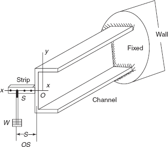
Figure 13.5 Shear centre
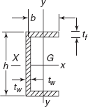
Figure 13.6 Channel section
OS = distance from centre of web to S at which no distortion takes place in the structural member.
Dimensions of the channel section are taken such as b = breadth of flange, h = depth of web, tf = thickness of flange, tw = thickness of web (as shown in Figure 13.6).
Theoretical value of shear centre distance

13.5 CREEP TEST
The aim of creep test on any material is to determine creep strain rate or the rate of time dependent part of strain. There are costly creeps testing machines on which steel samples can be tested at any constant stress at any temperature. But study of creep phenomenon can be easily done at room temperature and by using a very simple apparatus as shown in Figure 13.7. A lead wire of about 2–3 mm diameter of about 1 m length is taken. One end of the wire is wound at the steel hook fixed in the wall. At the other end of the wire a hanger with about 2 kg load is suspended and a wire is wound around the hook of the hanger. A steel scale is fixed in a clamp and arranged vertically. The scale is brought near the hanger with loads. Reading of the lower edges of the hanger is noted. The length of the wire between the hooks is measured. About 6–7 kg of load is gently placed on the hanger by holding the hanger. Now the load is gently allowed to hang freely on the wire. The instantaneous change in length dLo is noted. Ratio of dLo/L, i.e. the instantaneous strain, is shown on the graph between time and strain (see Figure 13.8). Initially, the strain rate is high and it gradually decreases to a constant value.
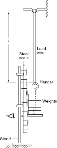
Figure 13.7 Creep test apparatus
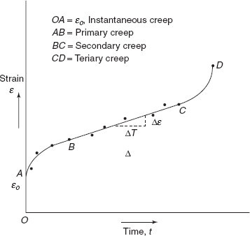
Figure 13.8 Strain vs time graph
Now the extension in the wire at intervals of 15 seconds is noted and after say 10 minutes, extension in wire (reading on scale) is noted at an interval of 1 minute. The change in length is continuously noted and it will be observed that change in length per unit time remains constant (during secondary portion of the graph).
After the constant strain rate, the strain rate abruptly increases. At this stage reduce the time interval for noting down the change in length. More readings should be taken near the stage of fracture of the sample. Now all the readings are plotted on a graph paper. The graph can be divided into three portions as shown in Figure 13.8. The first portion is Primary creep curve, wherein the strain rate goes on decreasing; second portion is secondary creep wherein the strain rate remains constant, and the third portion is tertiary creep in which the strain rate again goes on increasing till the wire breaks. Lead wire is very ductile and breaks with a conical-shaped fracture at the neck as shown in Figure 13.9. Slope of the curve during the secondary creep curve, i.e.
![]() , as shown, is defined as creep rate.
, as shown, is defined as creep rate.
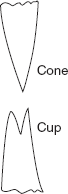
Figure 13.9 Lead wire failed in tension
- Remove the initial kinks, bends, etc. in the lead wire and try to make it straight.
- While winding the wire on the hook, see that no cut is made on wire.
- Gently release the load while starting the test.
- Note down the reading of change in length at regular intervals.
- Choose the amount of load depending upon wire diameter and time available for the experiment.
13.6 FATIGUE TEST
The aim of this experiment is to determine endurance limit of a material under cyclic loading, i.e. fatigue loading. Fatigue of metals is the property by which they fail at a relatively low value of stress when the stress cycle is repeated continuously. All the engineering components are subjected to loads during service. These loads need not be only steady loads. In most of the cases, these loads vary causing fluctuating stresses in the component. The material fails, once these fluctuating stresses reach sufficiently high values. The value of this stress may not be anywhere near the static strength of the material. This limiting stress which causes fatigue failure is called endurance limit stress. There can be any type of variation in stress cycle with time as shown in Figure 13.10; but the totally reversed stress cycle where σm =mean stress = 0 is the worst type of stress cycle. That is why fatigue strength of metals is generally determined under completely reversed bending conditions.
In the simplest type of machine for fatigue testing the load applied is of the bending type. The test specimen may be a cantilever or a simply supported beam. In the cantilever type the load may be applied at a single point or as simply supported beam load is applied at two points. When the load is applied at a single point, there is a tendency for failure of the specimen near the chuck. When the loading is applied at two points, a large volume of the test specimen is brought under the influence of load.
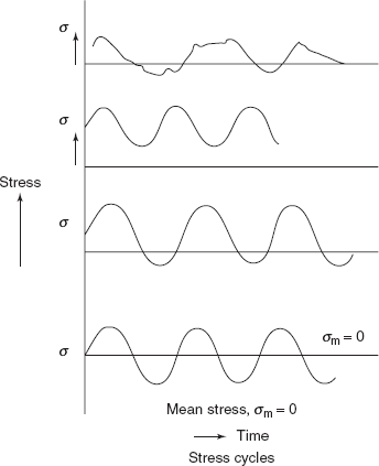
Figure 13.10 Various types of stress cycles
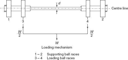
Figure 13.11 Specimen under four point loading
The simply supported beam type loading is made use of in the simplex rotating beam machine. The beam has an effective diameter of 7.62 mm. The long shoulders of the specimen are for mounting it on two sets of ball races, one on each side. The outer races serve as the supports and at inner races, specimen is loaded as shown in Figure 13.11. The specimen is rotated by an electric motor.
A large variety of testing machines are available in the market, each incorporating the following:
- A means for holding the specimen.
- A means for loazding the sample and measuring the load.
- An electric motor to rotate the specimen and a device to measure the number of revolutions.
- A means of disconnecting the revolution measuring device or pulling off the machine itself once the specimen is broken.
A number of standard test specimens are made from the metal under test. The first specimen is tested under high value of load. The number of revolutions the specimen experiences before fracturing is noted on the counter. Several specimens are tested with load decreasing for each specimen. Every time the revolution up to fracture is noted. The procedure is continued until a value of stress is reached when the specimen does not fail, say even after 10 million revolutions. Figure 13.12 shows the loads and supports on the specimen under fatigue testing. From this diagram, bending moment over the portion, BC
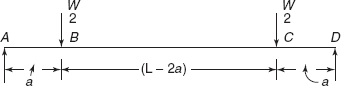
Figure 13.12 Specimen under four point loading
Say |
d = diameter of the sample |
|
σ = maximum stress in sample |
For each loading condition, maximum stress in sample s is worked out and corresponding number of revolutions up to failure of the sample are noted. Say these values are σ1, N1; σ2, N2; σ3, N3…σn, Nn are noted down. A graph is plotted between σ and N as shown in Figure 13.13. The stress at which the σ –N curve becomes asymptotic is known as endurance limit stress, σe.
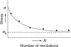
Figure 13.13 S-N diagram
Precautions:
- All the samples should be made from the same lot of the material.
- All the samples should be of exactly same dimensions or they should be made on CNC machines.
- Surface finish on all the samples should be of the same order.
- Environmental conditions should be maintained the same for all tests.
13.7 DETERMINATION OF YOUNG’S MODULUS AND POISSON’S RATIO
The aim of this experiment is to determine the value of Young’s modulus of elasticity and Poisson’s ratio of the material of the specimen such as mild steel, aluminium, copper etc. A specimen of the shape, shown in Figure 13.14, is made from flat piece. Then two electrical strain gauges in the axial direction ASG, two strain gauges in the lateral direction LSG, and two strain gauges on a piece of the same material, as dummy gauges DSG, are installed and cured and moisture proofed. Then leads are connected to all these six strain gauges. Gauge factor of the gauges is noted down. Sample is connected to a lever ABC, through links AD and EF as shown in Figure 13.15. At the end of the lever, at C, a hanger is suspended so that load can be applied.
Now connect the leads from these strain gauges to the terminals of A, B, C, D of a strain indicator. The experiment will be performed in two steps:
I Step: Two axial gauges ASG and two dummy strain gauges DSG are connected as shown in Figure 13.16. Strain indicator bridge is balanced and gauge factor is set on strain indicator. Loads are applied on the hanger one by one and readings of strain are recorded and plotted as shown in Figure 13.17. From the graph ΔW/Δεa is noted down.
where n = lever ratio.
Moreover, there are two active strain gauges ASG, therefore actual strain in axial direction is ![]()
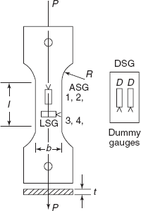
Figure 13.14 Flat sample with strain gauges
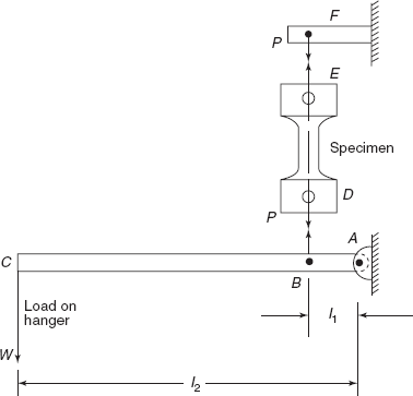
Figure 13.15 Loading of sample in tension
So, Young’s modulus, ![]()
II Step: Now two strain gauges in the lateral direction and two dummy gauges are taken and their ends are connected to four terminals A, B, C, and D of a strain indicator as shown in Figure 13.18. After balancing the bridge, setting the gauge factor knob, readings of lateral strain εt are recorded for various values of loads at the hanger and a graph is plotted as shown in Figure 13.19. Determine the slope of the graph, i.e. ΔW/Δεt. Then Poisson’s ratio,
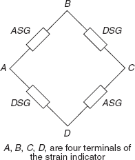
Figure 13.16 Strain gauges in strain indicator
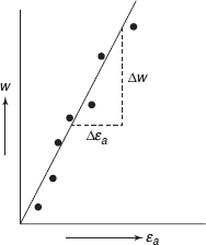
Figure 13.17 Load vs strain graph
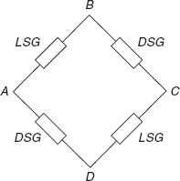
Figure 13.18 Strain gauges in strain indicator
i.e. ratio of the slopes of two graphs, i.e. lateral strain versus load and axial strain versus load, gives the value of the Poisson’s ratio of the material.
Precautions:
- The strain gauges must be properly cured and moisture proofed.
- Length of the leads in all the strain gauges must be the same.
- Leads must be tightly connected at the terminals.
- Bridge must be balanced at the strain indicator before taking the readings.
- Pointer on strain scale should be adjusted to zero in the beginning.
- Take the reading of the strain when it is stabilized.
- Set the gauge factor knob correctly.
- The leads should not swing while taking the readings.
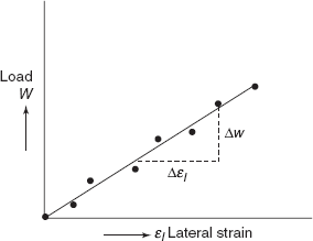
Figure 13.19 Load vs lateral strain graph
13.8 DETERMINATION OF SHEAR MODULUS
The aim of this experiment is to determine shear modulus of a material. In this experiment a hollow shaft of internal diameter d and external D is fixed at one end. At the other end, a lever is welded at the end of which load W can be applied as shown in Figure 13.20. Strain gauges are mounted along the neutral axis at an angle ± 45° as shown. Note that bending moment WL2 acts on the shaft and to eliminate the effect of bending moment and to record only the effect of twisting moment WL1 on the shaft, then, strain gauges are mounted along the neutral axis of the cantilever. Two strain gauges are also mounted on the other side of the hollow shaft, along the neutral axis.
say, τ = shear stress developed on the surface of the shaft.
Then principal stresses will be + τ and –τ at angles of ± 45° to the shaft axis. That is why the strain gauges are mounted along the principal stress directions so as to record principal strains.
If E is the Young’s modulus and v is Poisson’s ratio of the material, then principal strains are
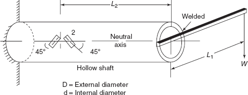
Figure 13.20 Pipe specimen under torsional loading
|
|
and |
|
i.e. |
ε1 = ε2 |
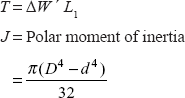
Gauge 1 will be in tension and gauge 2 will be in compression. Similarly the gauge 3 (in tension) and gauge 4 (in compression) can be located. These four strain gauges, i.e. two in tension and two in compression, are connected to the terminals A, B, C, and D of bridge of a strain indicator as shown in Figure 13.21. Bridge is balanced and strain scale pointer is adjusted at zero. Gauge factor knob is adjusted on the gauge factor of the strain gauges. Now the load is applied in steps at the hanger on the lever and reading of εnet is recorded.
Readings of W and εnet are recorded and plotted as shown in Figure 13.22.
From the graph slope ![]() is noted
is noted
Now torque on the shaft
Now
Figure 13.21 Strain gapes connected in strain indicator
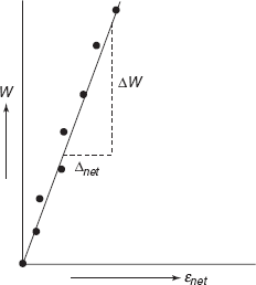
Figure 13.22 Load vs not strain
where τ is the shear stress on the surface
Substituting this value
Shear modulus,
Slope of the graph between W and εnet is accurately noted and shear modulus G is calculated as above.
Precautions:
- Apply the load slowly and gradually. Do not release the load from a height.
- The strain gauges must be properly cured and moisture proofed.
- Length of the leads for all the strain gauges should be the same.
- Leads must be connected tightly at the terminals of strain indicator.
- Take the reading of the strain when pointer is stabilized or reading on digital strain is stabilized.
- Lead wires should not swing while taking the readings.
13.9 CALIBRATION OF A PROVING RING
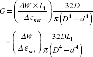
Proving ring is an apparatus used to calibrate testing machines. Basically it is a force transducer. There are various capacities of proving ring depending upon the mean radius, radial thickness, and width of the ring. Generally, there is a dial gauge fitted diametrically inside the ring. When there is diametral compression load on the ring, there is a deflection in dial gauge which is directly proportional to the load, and calibration constant depends on dimensions of the ring and elastic constants of the material of the ring.
In this experiment, there are four strain gauges mounted on the ring and output from these electrical resistance strain gauges is directly proportional to the applied load. Figure 13.23 shows the arrangement of strain gauges.
Strain gauges are mounted on the inner and outer curved surfaces of the ring as shown in Figure 13.24, along the horizontal diameter X X, i.e. centre of the strain gauges lies along x-x axis.
When the vertical load acts on the proving ring, inner gauges R1 and R3 are in tension, say tensile strain εt, and outer gauges R2 and R4 came under compression, say εc is the compression strain on R2 and R4. Gauges are connected in wheatstone bridge circuit as shown in Figure 13.25.
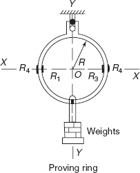
Figure 13.23
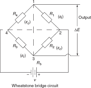
Figure 13.25
Strain gauge R1 is connected in arm 1–2, strain gauge R2 is connected in arm 2–3, strain gauge R3 is connected in arm 3–4, and strain gauge R4 is connected in arm 4–1 of the Wheatstone bridge circuit. Connections are made on strain indicator for full bridge. Gauge factor is set on the indicator and null balance is achieved, i.e. output ΔE = 0. Now load W is applied on proving ring and output reading is taken on strain indicator which is given as follow:
|
εnet |
= εt − (−εc) + εt − (−εc) |
|
|
= 2εt + 2εc |
Load is applied in variable steps and reading of enet is noted down on strain indicator. Readings are tabulated as given is Table 13.3.
Graph is plotted between load and εnet strain as given in Figure13.26. Slope of the straight line OA, passing through mean positions of observations, is termed as calibration constant.
Calibration Constant of Providing Ring = ![]()
Table 13.3 Readings of load vs not strain
S.No. |
Load on Proving Ring |
εnet |
|---|---|---|
1 |
w1 |
εnet1 |
2 |
w2 |
εnet2 |
3 |
w3 |
εnet3 |
– |
– |
– |
n |
wn |
εnetn |
Precautions:
- Apply the load on proving ring slowly and gradually.
- Strain gauges must be properly cured and moisture proofed.
- Length of the leads for all strain gauges should be the same.
- Leads must be connected tightly at the terminals of strain indicator.
- Take the reading of the strain when the pointer as strain indicator dial is stabilized.
- Lead wires should not swing while taking the readings.
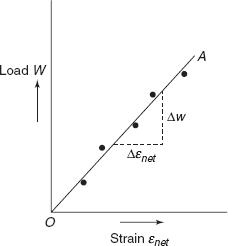
Figure 13.26 Calibration curve
13.10 CALIBRATION OF A PHOTOELASTIC MODEL FOR STRESS FRINGE VALUE
Though the stress fringe value for different photoelastic model materials is available in the literature but to accurately determine stresses in any photoelastic model, every batch of photoelastic material should be calibrated for stress fringe value fσ.
A plane circular disc of photoelastic material of known diameter D is taken. It is placed in loading frame of a circular polariscope. A dark field circular polariscope arrangement of polarizer, analyzer, and quarter wave plates is made, in which we obtain isochromatic fringes on model of order 0, 1, 2, 3,…, etc. The photoelastic model of circular disc is loaded under diameteral compression as shown in Figure 13.27. Loads are gradually applied on model, and isochromatic fringe order at the centre of the disc is noted and readings are tabulated as follows:
| P, Load on model | Isochromatic fringe order at centre of disc, N |
|---|---|
0 |
0 |
P1 |
1 |
P2 |
2 |
P3 |
3 |
P4 |
4 |
P5 |
5 |
P6 |
6 |
A graph between P and N as plotted and shown in Figure 13.28.
A straight line is passed through the mean position of the points plotted. Slope of the graph P versus N is noted. Figure 13.27 shows the isochromatic fringes on model when viewed at the end of analyser.
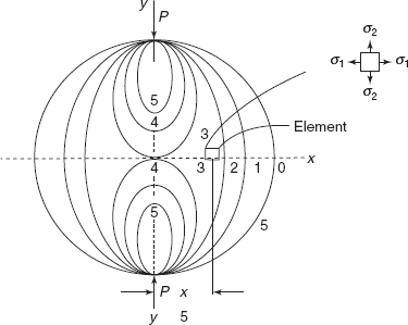
Figure 13.27 Disc under diameters compression
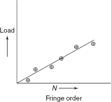
Figure 13.28 Load vs fringe order graph
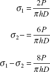
If we consider a small element at a distance of x from centre of the disc, then principal stresses at the point are:
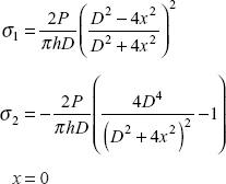
at the centre,
where |
D = |
disc diameter, |
|
h = |
thickness of disc, and |
|
P = |
diameteral load on disc. |
But
So,
or stress fringe value,
slope of ![]() is noted from graph (Figure 13.28).
is noted from graph (Figure 13.28).