3 A behavioral-institutional model of endogenous growth and induced technical change

Introduction

A fundamental tenet of conventional economic theory is that there is only one sustainable wage path to economic development and, in the long run, economies converge in terms of real per capita gross domestic product (GDP) and mean factor prices. Thus there can be no such thing as a high wage path to economic growth and development since convergence occurs through the process of interregional and international trade and factor mobility and is facilitated by the unfettered working of the marketplace.¹ But, the empirical evidence is heavily weighted in favor of the argument that convergence has not taken place internationally over time, with low and high income economies persisting side by side (Baumol 1986; Baumol and Wolff 1988; De Long 1988; Dowrick and Gemmell 1991; Olson 1996; Pritchett 1997). The absence of convergence raises theoretical and practical questions as to why convergence has not taken place. Moreover, contrary to both conventional and non- conventional models there is a negative correlation between either per capita income or per capita income growth and income inequality across nations, which contravenes the long held belief that income inequality and increases thereof are conducive to economic growth (Altman 2004b, 2008b; Aghion et al. 1999; Deininger and Squire 2008).

The alternative behavioral-institutional model of endogenous growth and induced technical change presented here, builds on the classic Solow growth model (1956, 1957, 1994; see also Jones 1998). My supply-side factor price-led (focusing on wage rates) model of growth provides a possible explanation for sustainable “equilibrium” differences in real per capita GDP, sustainable high wage growth, and relative income equality consistent with high per capita growth, even under the assumption of relatively competitive product markets. My alternative model, introducing more realistic behavioral and institutional assumptions embedded in efficiency wage and x-efficiency theory, yields dramatically different analytical predictions and understandings than conventional growth theory. This follows in the tradition of John Commons (1911, 1923; see also McIntyre and Ramstad 2002) in locating causality in economic outcomes in the design of economic institutions, with a special focus upon the labor market, labor rights, and bargaining power relationships (see also Rothschild 2002). In contrast, when conventional economics takes institutions seriously, its focus is largely on private property rights, following in the tradition of Douglass North (1971, 1990).

I argue that higher rates of growth are a positive function of market pressures, labor costs being most important, which induce technological change and x-efficiency as well as the institutional changes and public good investments necessary to the effective realization of such economic improvements. This modeling framework allows for at least two sustainable paths to economic growth even within the framework of competitive markets. At one extreme is the low wage path and at the other is a high wage path. The latter is associated with a higher level of equilibrium per capita real GDP and the former with a lower level.

In this model, convergence in real per capita output and real wages need not take place through the workings of competitive markets. Also, the high wage economy may also be characterized by a higher rate of growth. This would be a product of increasing levels of x-efficiency and higher rates of technological change induced by the relatively high wage regime. Moreover, this model is consistent with and helps explain the stylized fact of relatively more equal income distributions being correlated with higher levels of per capita income and higher rates of economic growth. Institutional parameters play a key background role in this model in that they can facilitate and promote or hamper or block technical change and improvements in x-efficiency.

The conventional growth model and amendments

Aspects of Solow’s analytical framework that is of particular interest to this chapter is the assumption that the long-run equilibrium level of per capita output is determined by an exogenously given propensity to save (where savings and investment are assumed to be equal) and the rate of exogenous technical change. The former yields the capital to labor ratio. Ceteris paribus, the more capital per worker, the more output per worker, subject to the stylized fact of diminishing returns. The long-run equilibrium growth rate in total output is given by an exogenously determined labor force growth rate plus the rate of exogenous technical change. The aggregate production function is characterized by constant returns to scale while all individual inputs are subject to diminishing returns.² Competitive markets are also assumed. So is long-run “full employment” given by Keynesian macroeconomic policies, a point often ignored in contemporary growth theory. Full employment policy maintains a stable macro environment wherein investment and employment rate are maximized.

Absent technical change, increasing capital per worker does not entail a sustained increase in the rate of growth in output per worker or per capita. Any positive gap between aggregate savings and the amount of investment required to keep capital stock per worker constant can only have a temporary effect on per capita growth. The increase in the rate of growth is transitory, sufficient to drive the economy to a higher level of output per worker and, ceteris paribus, to a higher level of per capita income. The transitory nature of growth is given by diminishing returns to capital. In equilibrium, the economy returns to a zero labor productivity growth rate.

These points, upon which the alternative behavioral-institutional model builds, are illustrated in Figure 3.1, where YW₀ is a production function and s(Q/L) is the corresponding savings function which equals the investment function (s is the savings rate, Q is output, and L is labor inputs). The amount of capital K and thus the new investment required to maintain a constant capital—labor (K/L) ratio is given by (n+d)*(K/L). This is the required capital function.³ The labor force growth rate is given by n and d is the depreciation rate. Note that (K/L) increases output per worker (Q/L) at a diminishing rate. The Solow equilibrium is given by the intersection of the investment and required capital function, such as at a′ given by K/L*. This yields an equilibrium level of labor productivity and thus per capita output, such as 0a. A higher savings rate (s) shifts upward the saving function to s*(Q/L) yielding a new higher level of labor productivity at 0b given by the higher equilibrium level of capital per worker. There is no permanent increase in the growth rate. Increasing n or d shifts upward the required capital function causing labor productivity to fall as a consequence of an equilibrium decline in the capital to labor ratio. In the long run, changing the independent variables has only a level effect on labor productivity. The long-run growth rate of labor productivity and, ceteris paribus, of per capita output, is always zero. In the Solow model the aggregate output growth rate is given by the full employment, employment growth rate, n.⁴

Figure 3.1 Determinants of output per worker.

In the Solow model, only continuous technological change yields sustained increases in output per worker. There is a limit to which savings can be increased and increasing capital is subject to diminishing returns. However, as Solow well admits (1994, p. 48), there is no clear causal mechanism in his model to explain the process of technical change and thus continuous per capita economic growth. Technical change shifts the production function YW₀ upwards to YW₁ for example, increasing the output to capital ratio [(Q/L)/K/L) = (Q/K)]. Continuous shifts in the latter yields sustained per capita growth. Otherwise, technical change has a one- shot level effect on labor productivity, yielding a short- run increase in growth until the equilibrium per worker growth rate of zero is restored at c′ (the savings function shifts upward to syT with technical change). In this model, unless all regions and nations are eventually characterized by an identical propensity to save and rates of technical change, which is what conventional wisdom suggests is true, convergence in per capita GDP growth rates is not expected and cannot be analytically predicted.

To address the potential paradox of non-convergence in the conventional worldview, the new growth theory, centered on the work of Paul Romer (1986, 1990; Aghion and Howitt 1998; Grossman and Helpman 1994; Helpman 1992; Lucas 1988; see also Barro and Sala-i-Martin 1995), assumes an aggregate production function characterized by increasing returns to scale from investment in knowledge (taking the form of research and development or formal education) as distinct from physical capital, where such investment has the problematic effect of increasing labor productivity without bound (Solow 1994, p. 50). The production function becomes convex or linear and one assumes away the demon of diminishing returns (Grossman and Helpman 1994, p. 35). Once the growth process is triggered through investments in knowledge, it becomes self-sustaining and leaders and laggards enter into sustainable path dependent equilibria. But since investment in knowledge is assumed to be characterized by positive externalities, it is possible for the market to underinvest in knowledge, generating less than “optimal” levels of per capita growth.

The new growth theory, however, does not provide us with an endogenous explanation of growth. Persistent differences in per capita GDP and growth between economies are products of ad hoc factors amongst which are different types of economic policy or historical accident.⁵ The new growth models are closed by exogenously determined institutional parameters.⁶ For this reason, the new growth theory leaves us no further ahead of the analytical game than Solow’s theory. Moreover, empirical work on the new growth theory does not provide strong support for the hypothesis that investment in knowledge is a fundamental cause for sustained economic growth and differentials in growth and per capita output between economies (Fagerberg 1994; Hall and Jones 1999; Mankiw et al. 1992; Pack, 1994; Solow, 1994). Also, there is no reason to expect investment in knowledge not to be subject to diminishing returns. In this sense new growth theory can be melded with the classic Solow model wherein such knowledge creation yields shifts in the production function, transitory increases in growth, and permanent levels effects on per capita income (Jones 1998).

Endogenous growth and induced technical change: the role of labor market pressures

X-efficiency and growth

A critical assumption of the alternative model, differentiating it from the classic Solow and endogenous growth models as well as heterodox models, is that wage rates—a proxy for wages, working conditions, and industrial relations—play a positive role in the growth process by affecting economic efficiency, innovation, and the adoption of extant technologies. In standard growth theories higher wages increase labor productivity only by inducing higher capital to labor ratios. But higher wages also increase unit costs and induce less employment, making the economy less competitive and reducing economic welfare.

Conventional theory assumes that economic agents are x-efficient and are thus maximizing both the quantity and quality of their effort inputs thereby maximizing output per unit of labor input. Once the assumption of x-efficient behavior is dropped, the predictions of the conventional neoclassical growth model are dramatically affected, giving way to a revised model that helps explain persistent differences in per capita GDP and rates of economic growth as well as movements of regions from leaders to laggards in the growth process and vice versa.

An important tenet of the original x-efficiency theory (Leibenstein 1966, 1979, 1982; Frantz 1988) is that in the absence of significant competitive pressure x-efficient behavior will be the exception to the rule. Unlike conventional theory, x-efficiency assumes that effort inputs vary with market structure and are only maximized when product markets are highly competitive. Also, given increases in x-inefficiency unit costs increase. This basic point is illustrated through equation (3.1).

In a simple model of the firm with one factor input, labor L, average cost AC equals the wage rate w, a proxy for all labor costs, divided by labor productivity Q/L. Any reduction in effort input reduces productivity Q/L and therefore increases unit costs AC. Increasing effort yields increases in labor productivity and lower unit costs. In the simple model, the percentage change in labor costs equals the percentage change in unit costs. When labor is only one of many inputs, as it is in the real world, average costs are much less affected by changes to labor costs. Movements in average costs are a function of the percentage share of labor to total costs—average costs change by the percentage change in labor costs times the percentage share of labor in total costs. This point is illustrated in equation (3.2):

where dAC is the change in average cost, dw is the change in the wage rate, and NLC is nonlabor costs. So, if labor costs are 20 percent of total costs, a 10 percent increase in labor costs only yields a 2 percent increase in unit costs (0.10*0.20=0.02). On the other hand a 10 percent cut in labor costs only generates a 2 percent reduction in unit costs.

In a modification to x-efficiency theory developed in detail elsewhere (Altman 1992b, 1996, 1998, 2001d, 2002, 2005b; see also Chapter 2), the level of x-inefficiency varies both in terms of market structure and the firm’s labor market environment (see also Akerlof 1984; Blinder 1990; Ichniowski et al. 1996; Kaufman 1989; Miller 1992). Increases in labor costs can be offset by increasing labor productivity through increases in the quality and quantity of effort inputs. Moreover, cuts to labor costs can result in offsetting cuts to labor productivity following from a drop in effort inputs. To the extent that higher wages and benefits (higher labor costs) induce sufficiently higher levels of x-efficiency and lower wages and benefits have the opposite effect, firms characterized by different labor costs need not be characterized by different average costs and firms characterized by different levels of x-efficiency need not be characterized by different average costs. In this model, movements in the level of x-efficiency can serve to offset the impact that movements in labor costs would otherwise have on unit production costs. Therefore, unlike in the conventional models and in the traditional x-efficiency model, increased labor costs need not result in higher unit costs and lower labor costs need not generate lower unit costs. In this scenario, even with highly competitive product markets x-inefficiencies need not be eliminated since x-inefficiency need not generate increases in unit costs.

In equation (3.1), when the percentage change in w is matched by the same percentage in labor productivity, unit costs remain invariant to changes in labor costs (w). If one introduces a more realistic model, as per equation (3.2), with more than one factor input, labor productivity need increase only by the percentage increase in labor costs scaled down by the share of labor to total costs. Labor need only retaliate marginally in response to cuts in income and benefits to prevent firms from becoming more competitive as a consequence of reducing labor costs.

In this alternative modeling, it is possible for x-inefficient firms to survive even with perfect product markets when wage rates differ between firms, if wages and related work cultures affect labor productivity by affecting the effort inputted into the process of production. Under these circumstances, low wage regimes would be causally related with low productivity and high wage regimes with high productivity, where the two different types of wage regimes need not necessarily yield any differences in unit costs or rates of return. One can, in effect, postulate a given level of average and marginal costs and rate of return to capital that correspond to an array of rates of labor compensation. There need not be any unique wage rate or labor compensation package that minimizes costs or maximizes the level of profits (Altman 1992b, 2001d, 2005b; Akerlof and Yellen 1990; Stiglitz 1987).⁷ In this scenario, low wage–low productivity and high wage–high productivity firms and economies can exist simultaneously and persist over time since there is no mechanism in place within the structure of the free market (perfect product market competition) to drive the wage rates and the levels of labor productivity toward convergence: low wage—x-inefficient firms do not have a competitive advantage over high wage firms, which can ultimately force convergence to take place. Indeed, low wages serve to shelter x-inefficient firms from competitive pressures. High wages are compensated for by higher productivity—higher levels of x-efficiency. On the other hand, if relatively high rates of labor compensation are not followed by sufficient increases in labor productivity, the high wage firms will, ceteris paribus, fall by the wayside in the process of inter-firm or international competition.

Some of these points are further illustrated in Figure 3.2. In the conventional neoclassical and x-efficiency models any increase in wages yield higher average costs as per line segment am. There is no positive causal relationship between labor costs and productivity. In the alternative model presented in this chapter (see also Chapter 2) as wages and related labor costs increase, average costs remain constant to the extent that average product (ah) increases sufficiently to offset increased labor costs as the level of x-efficiency increases (st). Up to 0b of labor costs there is an array of labor costs (proxied by the wage rate) consistent with a unique average cost of production 0a. High and low wage firms can be equally competitive in terms of unit costs. Effort inputs eventually hit the wall of diminishing returns where increasing effort inputs and related increases in labor productivity (hi) cannot offset increasing labor costs, yielding higher average costs (gc).

Firm decision makers have no immediate incentive to increase or cut labor benefits in this model in long-run equilibrium, once a particular wage rate is set.⁸

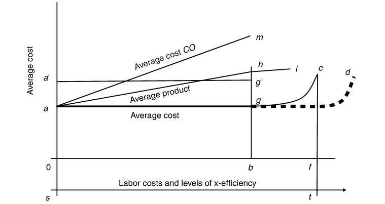
Figure 3.2 Unit production costs and x-efficiency.

Thus, there is a degree of path dependency built into this modeling framework. Members of the hierarchy do not derive any immediate benefits from increasing levels of x-efficiency and will only be supportive of long-run increases in labor benefits if their objective function incorporates their workers’ desire to increase their level of material well-being. On the other hand, cutting labor benefits yields no long term economic benefits to the firm (ag). But, cutting labor benefits might be pursued by firm decision makers whose utility is enhanced by increasing the relative gap between their income and that of their employees or who perceive that such policy will yield lower unit costs and higher rates of return.

However, in efficiency wage theory (Akerlof 1984; Akerlof and Yellen 1986, 1990; Bewley 1999), in the short run, firms might incur significant short term costs by reducing wages as workers retaliate by cutting effort inputs such that unit costs spike upwards in the short term (a′ g′). Only if the firm hierarchy perceives that such cuts are long term viable can one expect that low wage strategies will be pursued. The success of such a venture critically depends on the relative bargaining power between employees and employers. Therefore, a high wage regime might be an unstable one, contingent upon the preferences of members of the firm hierarchy and bargaining power considerations. The latter are affected by public policy with regards to labor mobility, bargaining and collective organizing rights, unemployment benefits, and the like, which affect the reservation wage rate and bargaining capabilities. From the perspective of this chapter, higher wages can positively impact upon growth since it positively affects productivity without increasing unit production costs. Lower wages negatively impact upon growth by lowering productivity.⁹

By increasing the level of x-efficiency and therefore the level of productivity, higher wages shift the production function in Figure 3.1 from YW₀ to YW₁, yielding a higher level of equilibrium productivity and ceteris paribus a higher level of per capita output. Given labor force growth and depreciation at 1 [(n+d)*(K/L)] and savings function s(Q/L), labor productivity increases from 0a to 0f′. If the savings rate remains constant then the production function shift also yields a shift in the savings function from s(Q/L) to s*(Q/L). This generates a higher level of capital per worker K/L** and an even higher level of labor productivity to 0g′ (Altman 2008b). There is no change in the long-run growth rate. But different levels of x-efficiency amongst economies yield long-run equilibrium differences in per capita output. There is no economic reason for convergence to take place under these circumstances.

More specifically, improvements to x-efficiency increases per capita income by increasing labor productivity and thereby the efficiency of capital and savings per capita given the ex ante savings rate. And this savings rate need not change even if the share of income going to labor increases as a consequence of increases in labor benefits. Much depends on differences in the propensity to save amongst workers and the economic elite and the extent to which corresponding tax changes yield the “old” savings rate. A decline in the savings rate need not reduce per capita savings from its original level, however, given the x-efficiency induced increase in per capita savings. Of critical importance in this model, are demand-side considerations. Aggregate demand must be such as to absorb the increased output generated by increases in x-efficiency. Consistent with the original Solow model proactive full employment macroeconomic government policy is assumed. In the absence of such policy, increasing efficiency will cause unemployment and might even have a negative consequence on growth.

In the first critical adjustment to the conventional growth model, effort becomes an argument in the production function and output becomes a function of effort per unit of labor input ε as well as of labor L, capital K, and “technical change,” where both technological change A and effort inputs ε are shift parameters. Effort inputs change as a function of labor market and institutional considerations, given by W.

The second related adjustment to the conventional model introduces technological change as a function of levels and changes to labor costs. In the fully adjusted revised model output becomes a function not only of capital and labor but also of labor costs and related institutional parameters that affect both the level of x-efficiency and the rate of technological change.

Induced technical change

In the model presented here, changes to and the relative level of labor costs play an important role driving technological change and can also impact in an important way on the investment in knowledge (the key variable in endogenous or new growth theory). Technological change is induced by key economic variables that, in turn, are impacted upon by institutional considerations. In this scenario, one can have differential technological change across firms and economics with no expectation of convergence with regards to technological change and related differences in per capita income. The revised model can be scripted as:

W refers to the absolute cost of labor or its relative cost.

I assume that increasing labor costs incentivize firms and economies to engage in technological change since otherwise (holding effort input constant) unit costs rise and rates of return fall. As per Salter (1960), I assume that firms (decision makers) are most concerned with minimizing costs when deciding on technological change irrespective of factor prices, ceteris paribus. But like Hicks (1932), Binswanger (1978), Hayami and Ruttan (1971), and Hayami and Ruttan (1973), for example, I assume that technological change can be affected by relative factor prices (for an historical take on this issue see Habbakkuk 1962 and Allen 2009, 2011). Increasing labor costs, relative or not, induces technological change.

To simplify the discussion, I assume that the type of output of all firms or economies is identical (one good model) and I only refer to relative increases in the price or cost of labor. In the model presented here, an increase in the relative price of labor has the immediate and short term effect of increasing the unit cost of production and reducing the rate and amount of profit. If the firm is to survive, however, ceteris paribus, an increase in the relative rate of labor compensation must be accompanied by a sufficient increase in labor productivity to offset this increase. Increasing the extent of x-efficiency is one means to this end. Technological change is another, although improvements in the former might be necessary to the latter.

High wage firms are forced to adopt already available technologies that are new to these firms. They may also find it worthwhile to develop new technologies (to innovate). Both such changes are components of technical change. The latter might require investment in on-the-job training and formal education by employees and the firm, redesigning existing plant, as well as research and development expenditure. Technological change shifts the production function upward. The low wage firms need not be so inclined. Low wage firms need not adopt the new technology or innovate if they can effectively compete on the basis of low wages. Moreover, the low wage regime may result in labor being too x-inefficient for the new technology to be cost effective.

This point is illustrated in Figure 3.3. Assume two economies I and J producing identical outputs using identical technologies at identical factor prices. The initial equilibrium for both economies is at A at isoquant Q₀, given isocost curve BC. The wage rate increases in economy I pivoting the isocost curve from BC to BC′ which is tangent to isoquant Q₁ at A*. Thus the high wage regime is more capital intensive than the low wage (given by the greater slope of ray 2 than ray

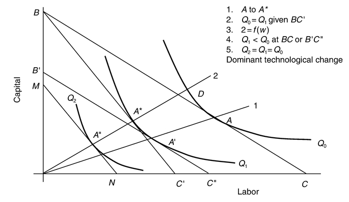
Figure 3.3 Labor and production costs.

1). Moreover, isoquant Q₁ represents a smaller amount of output than Q₀ while BC and BC′ represent the same level of expenditure. The initial level of output Q₀ can be produced at the higher wage (at D, the new factor price ratio) only at a higher level of expenditure and therefore at a higher unit cost. High wage economy I’s unit costs are therefore greater than low wage economy J’s. There has been induced technological change, of labor saving type, in the sense that firms change their cost minimizing factor input mix, from a known menu of techniques of production as relative factor prices change. But technical change does not take place in the sense of choosing or developing a technology that maintains or reduces ex ante unit costs. If all factor prices increase proportionally, yielding a parallel move inward of the high cost economy’s isocost curve to B′C″ from BC, the old budget yields a lower level of output and the old level of output (Q₀) can only be produced with more expenditure and therefore at a higher unit cost. In this scenario, high wage firms cannot economize by reallocating factor inputs since there is no change in relative factor costs.

For the high wage economy to survive, assuming away for the moment the possibility of affecting the degree of x-inefficiency, more aggressive technical change must take place. For example, if Q₁ embodies the new technology such that output at Q₁ equals output at Q₀, unit costs in the high wage economy would be equal to unit costs in the low wage economy. In spite of the increase in labor costs, unit production costs remain unchanged as a consequence of technological change wherein the original level of output Q₀ can be produced with fewer inputs at Q₁. In terms of Figure 3.2, the average cost curve agc shifts to agd. Technological change allows for even higher levels of wages and related benefits to be consistent with a particular level of unit costs. The low wage economy, however, need not adopt the new technology to compete if its unit costs are the same as in the high wage economy. If, however, the new technology adopted by the high wage economy is represented by isoquant Q₂, where the level of output here equals that at Q₁, unit costs in the high wage economy diminish, given by the isocost curve moving from BC′ to MN. The low wage economy would be pressured to adopt new technology since, otherwise, unit costs in the high wage would be less than in the low wage economy. Such a technology, which both high and low wage economies must adopt to remain competitive, absent protection, I refer to as a dominant technology. High wage firms and economies would lead the process of technological change in this scenario. In all of these cases the high wage regime is more productive than the low wage regime. But apart from superior technologies, there are no good cost competitive reasons for the low wage economy to engage in technological change.

However, it should be noted that, ceteris paribus, the high wage induced technological change given by Q₁, if adopted by the low wage economy J, should yield lower unit production costs than what characterized post-technological change the high wage economy I. The low wage economy could produce Q₁ of output with a budget given by B′C″ whereas the high wage economy can produce this level of output at higher aggregate cost given by BC′. The high wage economies would here lead the process of technological change, with the low wage economies following. But there is no competitive imperative for the low wage economies to follow the leader as long as they remain cost competitive with the old technology. However, if the low wage firms followed the technological change lead, they would drive unit prices downward, forcing the high firms into a positive spiral of improvements in x-efficie ncy and technological change. Once again, the high wage firms and economies lead the process of technological change. In this scenario whether or not low wage firms adopt the new technology is contingent upon the objective function of firm decision makers; whether for example they are interested in increasing market share and increasing firm income by reducing unit price.¹⁰

However, the low wage regime may not be capable of exploiting the new technology as x-efficiently as the high wage economy. An important point by made by Leibenstein (1973) is that there might be a strong causal relationship between x-efficiency and technological change. Technological change might only be economically viable in a relatively x-efficient environment.¹¹ In conventional treatments of technological change, effort inputs are exogenously determined and not part of the technical change causal narrative. Nor are the costs involved in engaging in technological change paid much heed. However, technological change is costly and requires skill sets and motivational parameters absent in low wage economies. A high wage environment might be necessary to generate the synergies to make the new technology economically viable. Technological change may not be viable in a low wage regime when the new technology can only increase productivity if effort inputs increase, and this cannot transpire in the low wage environment. The new technology only yields the necessary increases in productivity to become economically viable under particular x-efficient environments. Low wage firms cannot be expected to adopt new technology yielding the same productivity as the old. Technological change is a non- starter if productivity actually diminishes as a consequence of an x-inefficient environment. For reasons of x-inefficiency, shifting to the new technology may not make the low wage economy any more competitive.¹²

In Figure 3.3, although technical change yields isoquant Q₁ (which equals Q₀ in output) in the high wage environment, the x-inefficiency effect of the low wage environment yields isoquant Q₀ where the latter is characterized by the same productivity features as the pre-technological change isoquant Q₀. The x-inefficiency effect here equals the productivity effect of technological change. There is no incentive for low wage firms to engage in technological change. And this ignores the cost involved in purchasing new plant and equipment and reconfiguring the shop floor, which typically goes hand in hand with technological change.

At a more general level, Nathan Rosenberg argues with respect to the process of technological change that “there is a threshold level at which the costs of the new technology become competitive with those of the old” (Rosenberg, 1982a, p. 27). Cost minimizing firms will not engage in technical change unless firm decision makers expect that such change will yield lower costs. In the model presented here the level of x-efficiency impacts on the effects that technical change have on unit costs. Also, more productive technologies need not yield lower unit costs when higher levels of labor benefits are necessary to the realization of higher productivity potential of the new technology. Yet, in his scenario, technological change is material welfare improving in that it yields Pareto improvements to the material well-being of employees.

Even where technological change is consistent with maintaining the competitiveness of the firm, decision makers might require inducements to engage in such Pareto improving technological change if this is not consistent with their objective functions. Adopting the new technology may involve both net financial and utility related costs (such as more time and effort and increased stress) to the firm hierarchy, at least in the short run. If the time horizons of members of the firm hierarchy are not especially long, technological change will not be utility maximizing and will be avoided. In addition, an argument in the decision makers’ utility function can be its relative income and power relative to employees, which can be diminished in the high wage firm. The low wage economy can also respond to the competitive challenge presented by technical change by forcing wage rates downward. Low wages can serve as a substitute for technological change. The effectiveness of the latter strategy depends, of course, on the impact that a fall in labor compensation has on the level of x-inefficiency. For these reasons, technological change is not inevitable. The absolute and relative rate of labor compensation can play an important role in determining the timing, the extent, and the rate of technical change through its impact on x-inefficiency.

In this model, as a consequence of labor market pressures, technological change shifts the production function upward as in the Solow model, in Figure 3.2 from YW₀ to YW₁. These shifts are predicted to take place given the capital—labor ratio; that is even if the capital to labor ratio does not change. The production function also shifts outward as the capital—labor ratio increases as function of an increase in the relative price of labor. Here we would have both shifts in and movements along the production function. In both scenarios, there is a resulting equilibrium increase in labor productivity and thus in per capita output and a short term increase in economic growth. Productivity and per capita income are further increased if saving propensities remain the same, shifting the savings function upward to syT.

In the long run, per worker and, ceteris paribus, per capita growth converges to zero and aggregate growth to that of employment (n). Sustained growth requires sustained inducements to improvements in x-efficiency and technological change. In this model, high wage economies lead the process of induced technological change as firms are motivated to adopt extant technologies and develop new ones in the face of labor market pressures. Low wage economies need not engage in technological change given the costs of so doing and, therefore, need not be at a competitive disadvantage over the high wage economies that have adopted extant and new technologies. This would even be the case of competitive product markets where identical information of technology is available to all firms. In this sense, both the high and low wage path to economic growth and development are sustainable in the long run.

Inadequate competitive pressures (inclusive of protection to high cost firms) can be expected to reduce the probability of technological change in low and high wage economies. Increasing competitive pressures, ceteris paribus, yields more technological change as Parente and Prescott (2000) suggest. Firms and economies are pressured to shift to low cost techniques of production as opposed to rent-seeking activities where high wage firms and economies can export their products at a relative low price. But market pressures can go only so far. The x-inefficiency generated by a low wage socio-economic environment obviates the need for technological change when such change does not reduce unit production costs. Even with highly competitive product markets technological change will not occur to the same extent in high and low wage economies and some technological gap can be expected to persist between high and low wage economies.

This point can be illustrated in Figure 3.4, where LW is the production possibility frontier (PPF) for a low wage economy protected from competitive pressures. Reducing protection results in firms adopting superior (cost reducing technologies), shifting the PPF to RP. The latter shift presumes that this economy is vested with the institutional parameters, inclusive of appropriate threshold levels of private property rights, necessary for the investment in technological change. Moreover such economies must be characterized by the capacity to identify and adapt least cost technologies to local circumstances. As Rosenberg argues: “Perhaps the most important single factor determining the success of technology transfer is the early emergence of an indigenous technological capacity. In the absence of such a capacity, foreign technologies have not usually flourished” (1982a, p. 171; see also Rosenberg 1982b).

What the modeling narrative in this chapter suggests is that this shift of the PPF is only part of the story and will not yield convergence in per capita income.

Figure 3.4 Production possibility frontier and institutional parameters.

Further sustainable per capita income gaps will remain until x-efficiency in production and related laggard performance in terms of technological change are eliminated. Improvement in labor market conditions will cause the production possibility frontier to shift further to XEXE′ (the relatively x-efficient PPF) and again to TfTg (the x-efficient technological change related PPF). Even in the absence of increasing product market competition, increasing labor market pressures (and improvements in labor market conditions) will yield outward shifts in the PPF from RP to XEXE′ for example. Economies such as China’s and India’s have experienced significant economic growth most recently as a product of opening up local markets to foreign competition and investment and providing increasing levels of private property rights. The model presented here suggests that these important economic advances will be limited by the extent to which private property rights as well as labor market pressures and, closely related to this, labor and democratic rights, remain limited. From this perspective, China might be facing more severe institutional obstacles to future growth than India.

Figure 3.5 illustrates more specifically the relationship between labor market parameters and per capita output underlying the alternative model. In quadrant I simple labor market relationships are specified. For this quadrant the vertical axis measures wages and related labor costs (W). For quadrant II, this axis measures output Y, which is some positive multiple of W. If one begins with equilibrium e₀ and labor costs W₀, this is causally related with thick PPF gg. Given employment and the employment to population ratio, a particular PPF is consistent with specific level of per capita output and as the PPF changes so does the level of per capita output. The thick PPF represents the possibility that for any given wage there is an array of outputs consistent with different levels of product market competitiveness. As product markets become more competitive, one moves from the inner to the outer boundary of the PPF.

Figure 3.5 Labor markets and output.

That which increases demand, given labor supply, yields an increase in labor costs. For example, a shift in demand from LD₀ to LD₂, given supply curve LS₀, yields an increase in the equilibrium wage from W₁ to W₂. This serves to shift the PPF outward to ffas a function of improvements in x-efficiencies and technological change.¹³ As long as institutions are not in place which restrict the capacity of workers to bid wages up, tighter labor markets have the effect of not only improving the conditions of labor but also serve to trigger one-shot increases in growth and permanent level increases in per capita output. This is why improvements on the demand side, inclusive of globalization, have the potential to improve the conditions of labor and wealth of nations, irrespective of the world-view of employers.

Conventional growth theory pays no heed to such demand-side issues.¹⁴ But this point was well recognized by Adam Smith (1937, p. 68) and is of particular importance to John Commons (1911). Macroeconomic policy that serves to tighten the labor market contributes to supply-side related wage-led growth, wherein higher wages incentivize economic actors into being more x-efficient and engaging in technical change. Any negative demand-side shock, such as a reduction of exports or a tightening of domestic demand, can be expected to have the opposite effect. A downward shift in demand to LD₀, for example, yields a fall in the wage to W₀, causing an increase in the extent of x-inefficiency and a reversion to less advanced technology. Here one has an inward shift in the PPF to hh from gg.

On the supply side, a tightening of the labor market, which can be illustrated by an inward shift of the supply curve such as from LS₀ to LS₁, has the effect of increasing the wage and shifting outward the PPF through its x-efficiency and technological change effects. Such improvements in the bargaining power of labor can be a product of severe demographic change, such as the infamous Black Death of fourteenth century Europe which wiped out a large percentage of Western Europe’s population or more benign institution changes, such as legalized labor mobility (the abolition of serfdom and slavery, for example), the development of unions, and the introduction of social safety nets such as minimum wages and unemployment insurance (Domar 1970; Altman 2000c, 2004a, 2005b). On the other hand, ceteris paribus, large increases in the supply of labor can negatively impact on the level of x-efficiency and the rate of technological by forcing wage rates downward. Also, institutional changes, which reduce the bargaining power of labor, serve to reduce the equilibrium wage. This can be illustrated by the extreme case of supply curve LS₂, where any increase in demand has no impact of the equilibrium wage.

Embodied "Kaldor" technological change

Kaldor maintains that both capital accumulation (increasing the capital to labor ratio) and technological change are intractably related with technological change embodied in the former (Kaldor 1957, 1961). In the model presented here, I retain the Solow assumption that one can isolate, empirically, the unique contribution of capital accumulation to increases in labor productivity. But this does not assume that technological change is independent of capital accumulation. Technological change typically requires investment in plant and equipment and often in human capital as well. In other words, in a dynamic modeling framework, increases in the capital to labor ratio might also result in shifts outward in the production function if such investment results in technological change.

In the model presented here, labor market pressures are predicted to induce improvements in x-efficiency and technological change where the latter requires investment. Given the facilitating relationship between capital accumulation and technological change, increasing labor pressures can be expected to increase the capital–labor ratio (a movement along the production function in Figure 3.2) and a shift in the production function as a consequence of improvements in x-efficiency and induced technological change. Embodied technological change can take place with respect to both net and gross investment since both replacement and “new” investment can embody technological change. Overall, given that technological change is embodied in net and gross investment, one can expect a strong positive correlation between investment and per capita economic growth (Jones 1998, p. 29; DeLong and Summers 1992; Wolff 1991) and for the strength of this correlation to increase where the micro inducements for technological change and improvements in x-efficiency are stronger.

This model is also consistent with related insights of Salter (1960; see also Bloch and Madden 1995) on embodied technological change wherein the latter is affected by the vintage of capital stock and its heterogeneous age composition. Older less productive capital stock embodying old technology is kept in place as long as it yields products that are competitive, slowing down the process of technical change. In the induced model presented here, labor market shocks induce a faster rate of replacement of capital stock and improvements in the level of x-efficiency of the vintage capital stock. When the older vintage capital’s improvements in x-efficiency no longer suffice to keep firms competitive, technological change can be expected to take place.

Saving, inequality, and the high wage economy

It is important to note that high wage induced x-efficiency and technological change yield more aggregate savings if the average propensity to save does not fall, in spite of the fact that wages and labor benefits increase. The production function shifts outward as wages rise as long as induced increases to productivity suffice to maintain aggregate savings per labor input. This shift is even greater if the average propensity to save does not change.

If the income of wage earners increases by more than other income groups, the average propensity to save does not decline if the average propensity to save of wage earners equals the social average in a two-class model of the economy (employee and employers). In a multi- income class model, even if the average propensity to save of workers is less than the social average, the average propensity to save does not diminish if the relative size of the middle income group (in a three income class model) increases sufficiently with increasing wages, and the average propensity to save of this income group exceeds that of the lower income group.¹⁵

If labor income increases relative to that of other income groups, as it would where higher wages and labor benefits motivate improvements in x-efficiency and technical change, income inequality diminishes. But given no negative impact on aggregate savings per labor input, high wage growth is consistent with a lessening of income inequality when measured by the income of wage earners relative to that of employers and other members of the firm hierarchy. As already mentioned increasing income equality need not result in reducing savings per labor input or the average propensity to save; there might even be an increase in the values of these two variables.

The revised model and new growth theory

In the revised model, unlike in new growth theory, research and development (R&D) expenditure and investment in human capital are subject to diminishing returns (see also Jones 1998). Therefore changes in these variables yield only short- run increases in growth rates and one-shot increases in per capita income. In this model, there is no reason why R&D need generate technological change (Ruttan 1997). It might very well yield new or improved technology. But firms need the incentives to adopt or adapt such technology.

In the induced growth model, labor market pressures induce firms to invest in R&D and to engage in technological change. In addition, even if there is little R&D in a firm or a particular economy, significant technological change can take place as labor and related costs increase. Firms here have the incentive to adapt the innovations of others to remain competitive. And, technological change need not take place even if there is significant R&D if the appropriate incentives are not present to engage in technological change. As an example, leaders in R&D, such as the United States, in the recent decades have not been leaders in technological change (Parente and Prescott 2000; Jones 1998, p. 156).

Finally, human capital formation requires incentives if it takes place on the initiative of the state, firms (training), and individuals. High wages can create such incentives. In institutional environments where low rates of return are expected, one cannot expect much privately initiated human capital investment. Moreover, when human capital investment takes place in such an environment, it can be expected to be relatively unproductive, contributing little to augmenting the permanent level of per capita income. This would be the case even if the state heavily subsidizes human capital investment. In the model presented in this chapter, labor market pressures shift the production possibility curve outward, in terms of their effect on R&D and R&D related technological change and on human capital formation, yielding permanent level effects on labor productivity and short term effects on the rate of economic growth.

Sustainability of high wage growth

The high wage regime might be more unstable than a low wage regime in so far as corporate leaders might have a preference for the latter and have the capacity to undermine the high wage regime by political means or by transferring location to low wage regions. Thus, preferences of corporate leadership, given that firms can produce competitively in a high or low wage environment, can play an important role in affecting the stability of high wage regimes (Bluestone and Bennett 1990; Perelman 1993). This is particularly true if an economy approaches the neoclassical ideal of perfect competition, with perfect mobility of capital and the absence of tariffs. But such is rarely the case in reality. Footloose industries would be more prone to this particular problem. High wage industries tied to a region or country for geographical, economic (transportation cost, economies of scale) or political reasons would be more stable. Adding to the stability of high wage regimes would be weak property rights and governance in low wage regimes, wherein the weakness in the latter two variables increase the risk of doing business in such economies.

A high wage regime would also be difficult to sustain if the necessary infrastructure to maintain a high level of productivity is not established. This includes the educational, R&D, health, legal (which incorporates but goes well beyond private property rights), good governance—of which democracy is a vital vehicle—and transportation and communication infrastructure which Moses Abramovitz (1986) refers to as a nation’s “social capabilities” (see also, Acemoglu et al. 2001; Altman 2008c; Diamond 2008; Easterlin 1981; Hall and Jones 1999; North 1990; Olson 2000; Rosenberg 1982a; Sen 2001). Social capabilities might differ across nations in important ways (Rodrik 2007). With respect to the legal environment, little attention has been paid in the literature to democratic rights, and labor rights specifically, as being an economically significant positive variable in driving the rate of growth. Attention has been focused on private property rights (North 1990; Olson 2000). But evidence suggests that sustained high rates of growth require secure property rights plus democratic rights, where the latter contributes toward incentivizing the growth process by facilitating a high wage environment and good corporate governance (Altman 2008a, 2008c; Sen 2001).

High wages may induce governments to engineer the social capabilities necessary for the high wage regime to be competitive. A low wage regime may have the opposite effect on government. In other words, labor market pressures can play an important role in inducing institutional change in the direction of facilitating and promoting high wage economic growth. Thus, positive labor market pressures can be expected to induce decision makers into reconfiguring institutions so that higher wage economies remain competitive (Altman 2006d, 2007, 2008a). On the other hand, adequate social capabilities per se are not sufficient to induce high rates of economic growth and high levels of real per capita output. On a microeconomic level, high wages are necessary to induce firms to become more x-efficient and to adopt more productive technology.¹⁶ Entrepreneurs, for example, must be incentivized into making x-efficiency augmenting and technological change related decisions.¹⁷ Rent-seeking decisions might be equally profitable, cost effective, and utility maximizing as economically efficient ones in a relatively low wage and protectionist environment. Thus, if the state can neutralize labor market pressures, the inducements for improvement in x-efficiency and technological change need not take place (Altman 2006c, 2007; Domar 1970; Lane 1958; North 1990; Olson 1996, 2000).

High wage growth is also subject to significant vulnerabilities when labor markets are not structured to provide firm owners, investors, and entrepreneurs with incentives to invest in plant and equipment and engage in technological change. Therefore, it is important to note that in this chapter high wage regimes refer only to relatively high mean (average) wage economies. High wage regimes does not assume the inflexibility of wages and labor costs in general in face of changes in the relative demand for labor in the different sectors of the economy. Nor does it assume the inability of firms to dismiss employees with cause or to the absence of secure private property rights and the related incentive environment necessary for entrepreneurs to flourish. These three capabilities are essential to dynamic entrepreneurial capitalism which is critical to transforming R&D and human capital investments into productivity enhancing economic activities (Baumol et al. 2007; see also Acs and Armington 2006; Audretsch et al. 2006).¹⁸

Not only are flexible labor markets compatible with high wages, but some of the institutional variables that contribute to relatively high wages (reservation wages) serve to facilitate the stability and sustainability of flexible labor markets. As Baumol et al. (2007) argue:

Such an economic construct, referred to by some as flexicurity, is characterized by flexible labor markets, strong private property and labor rights, a strong social safety net, high mean wages, and low unemployment rates (Kuttner 2008).¹⁹

Unlike many heterodox and mainstream models, in the model presented here high wages need not present an impediment to the growth process by squeezing profits by increasing unit production costs. Indeed, higher wages tend to induce increases in productivity yielding higher rates of growth. High wage led growth increases the level of potential per capita output at any point in historical time. Whether this induced increased productivity related growth is sustainable in the long run hinges upon the effectiveness of demand-side management in absorbing increased output and maintaining “full employment.” Sustainable and optimal high wage growth requires macroeconomic policy configured to maintain full employment and thus minimizing the difference between potential and actual unemployment. Macro policy not oriented toward full employment reduces the equilibrium level of per capita output on the demand side, but also reduces labor market pressures thereby reducing the level of potential per capita output on the supply side (on the multi-faceted demand-side literature see, Altman 2003b, 2006d; Bhaduri and Marglin 1990; Bhaduri 2008; Dutt 2006; Madrick 2007; Maddison 1982; Özlem and Stockhammer 2008; Özlem and Yentürk 2001; Rowthorn 1981).²⁰

Conclusion

A central objective of this chapter is the development of a reasonable theory of induced economic growth by introducing wage rates to the Solow model as a positive causal determinant of x-efficiency and technological change. The revised model is endogenous in so far as labor market conditions and other institutional parameters are part of the economic system. But the model is closed by institutional variables, which must ultimately determine the state of the labor market. This highlights the importance of, for example, both labor and property rights as determinants of per capita income and growth.

This behavioral-institutional model helps explain the origins of important and stable differences in per capita income and growth rates across economies and thus the persistence of both high and low wage economies over historical time even in a highly competitive environment. One can also explain significant variations in income inequality for given levels of per capita income and high levels of per capita income and growth being consistent with relatively low levels of income inequality. Moreover, it is now possible to more clearly explain how an economy can revert from leader to laggard in the growth and development process. Whether or not convergence takes place depends on the state of the labor market and on the extent to which an economy can sustain relatively high rates of labor compensation.

Labor market conditions varying across firms and economies can yield persistent and sustainable gaps in per capita income. This is not to say that other factors, both endogenous and exogenous, are not important to explaining this phenomenon. However, in the tradition of John Commons, by focusing on the level and relative rate of labor compensation, one is isolating an easily identifiable and measurable as well as significant economic variable as a possible supply-side determinant of the growth process. This variable has typically been ignored in the literature as a determinant of technical change. Moreover, it has not been causally related to levels of x-efficiency which, in turn, can have a significant impact on the extent of technological change. All told, the alternative theory helps explain persistent differences in levels of material well-being across firms and economies and why firms and economies can remain well below their productive potential over time even in the face of severe competitive pressures. Institutional parameters are critical to such an explanation.