Chapter 6
Time Dependence in the 1-D Models
In Chapter 5, we found that time-independent, zonally symmetric models can be cast into the form of a linear differential equation in the latitude variable with zero-flux boundary conditions at the poles. In the case of a latitude-independent thermal diffusion coefficient, the system can be solved with Legendre polynomials. In this chapter, we extend this procedure to the case of time dependence. Such an extension allows for idealized seasonal-cycle simulations for the zonally symmetric planet. Introducing time dependence necessarily requires some kind of effective heat capacity for the column of air–land or air–ocean medium. When we take the planet to have a homogeneous surface and constant diffusion coefficient, we also specify that the heat capacity is not spatially dependent, that is, it is a constant. An all-land planet is one for which the heat capacity is characteristic of a land surface. This means it takes a value calculated from a fraction (nominally half) of the mass of a column of air. This leads to a time constant ![]() of about 1 month. This is our new phenomenological coefficient for Chapter 6.
of about 1 month. This is our new phenomenological coefficient for Chapter 6.
The time-dependent models are amenable to analytical solution for uniform planets (constant ![]() and
and ![]() ). Model solutions are in the form again of Legendre polynomial modes, each having a characteristic decay time with larger scales (low Legendre index) having longer relaxation times, and smaller scales, shorter times. The seasonal cycle of latitude-dependent insolation has a very simple form when truncated at the few-mode level. Legendre polynomials of index 0, 1, and 2 describe the latitude dependence of the seasonal cycle of insolation, except, of course, for the discontinuous derivative near the poles, which is necessary to describe the onset of perpetual night or day and the appropriate latitudes and times of year. This insolation formula allows us to obtain very simple expressions for the dependence of insolation on obliquity, precession of the equinoxes, and eccentricity. The seasonal cycle simulations also give us an idea about the lag of seasonal response to the driving seasonal heating cycle.
). Model solutions are in the form again of Legendre polynomial modes, each having a characteristic decay time with larger scales (low Legendre index) having longer relaxation times, and smaller scales, shorter times. The seasonal cycle of latitude-dependent insolation has a very simple form when truncated at the few-mode level. Legendre polynomials of index 0, 1, and 2 describe the latitude dependence of the seasonal cycle of insolation, except, of course, for the discontinuous derivative near the poles, which is necessary to describe the onset of perpetual night or day and the appropriate latitudes and times of year. This insolation formula allows us to obtain very simple expressions for the dependence of insolation on obliquity, precession of the equinoxes, and eccentricity. The seasonal cycle simulations also give us an idea about the lag of seasonal response to the driving seasonal heating cycle.
Later in the chapter, we return to the stochastic nature of climate forcing (presumably due to weather instabilities) by showing how the random walk of heated parcels is approximately imitated by diffusion in an ensemble average. This analysis relates the mean square of the parcel's velocity and relaxation time to the diffusion coefficient of the ensemble.
A short section is added to show how one might go about solving one-dimensional problems via finite difference methods. The appendices to the chapter givederivations of the insolation functions.
6.1 Differential Equation for Time Dependence
Consider the problem of a time-dependent one-dimensional climate system for a planet whose surface is uniformly land or ocean. The energy balance model for constant coefficients is as follows:

where ![]() is the
is the ![]() (latitude),
(latitude), ![]() is time,
is time, ![]() is the latitude and time-dependent temperature field,
is the latitude and time-dependent temperature field, ![]() is the insolation function possibly allowing for a seasonal cycle,
is the insolation function possibly allowing for a seasonal cycle, ![]() is the coalbedo, which is a function of latitude and possibly time dependent;
is the coalbedo, which is a function of latitude and possibly time dependent; ![]() is the total solar irradiance divided by 4 =
is the total solar irradiance divided by 4 = ![]() ,
, ![]() , and
, and ![]() are phenomenological coefficients as defined in Chapter 5, and
are phenomenological coefficients as defined in Chapter 5, and ![]() is an effective heat capacity. As discussed in Chapter 2, this means a timescale of about 30 days (
is an effective heat capacity. As discussed in Chapter 2, this means a timescale of about 30 days (![]() ) for an all-land planet and a few years for a planet covered with a mixed-layer ocean. This amounts to using the heat capacity of half a column of air (at constant pressure) for the all-land case and that of 50–100 m of water for the mixed-layer ocean case. In the latter, we assume the ocean below is uncoupled with the mixed layer.
) for an all-land planet and a few years for a planet covered with a mixed-layer ocean. This amounts to using the heat capacity of half a column of air (at constant pressure) for the all-land case and that of 50–100 m of water for the mixed-layer ocean case. In the latter, we assume the ocean below is uncoupled with the mixed layer.
We expand the time-dependent temperature field into Legendre polynomials:
Note that each coefficient ![]() is a function of
is a function of ![]() . After inserting the series, multiplying through by
. After inserting the series, multiplying through by ![]() and integrating as before we obtain an ordinary differential equation for the
and integrating as before we obtain an ordinary differential equation for the ![]() :
:

where

It is important to note that none of the terms in the array indicated by (6.3) is coupled to any of the others. In other words, for the equation dependent on mode number ![]() there is no other mode index, say
there is no other mode index, say ![]() , that is referred to in the equation indexed by
, that is referred to in the equation indexed by ![]() .
.
6.2 Decay of Anomalies
Consider first the case where ![]() and
and ![]() are set at their mean annual values as in Chapter 5. We can examine the behavior of the climate as it is perturbed away from steady state. We have the solution to the initial-value problem:
are set at their mean annual values as in Chapter 5. We can examine the behavior of the climate as it is perturbed away from steady state. We have the solution to the initial-value problem:
where ![]() is the solution to the time-independent (steady-state) problem given above and
is the solution to the time-independent (steady-state) problem given above and

Each mode ![]() has its own characteristic time
has its own characteristic time ![]() . Note that the characteristic times fall off rapidly as a function of
. Note that the characteristic times fall off rapidly as a function of ![]() as shown in Figure 6.1. This agrees with our intuition that larger spatial scales have longer characteristic (adjustment) times. We will establish a similar result for the autocorrelation times later in noise-driven models.
as shown in Figure 6.1. This agrees with our intuition that larger spatial scales have longer characteristic (adjustment) times. We will establish a similar result for the autocorrelation times later in noise-driven models.
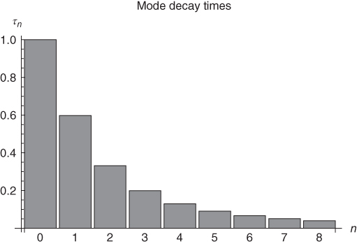
Figure 6.1 This figure illustrates that large spatial scales (low Legendre index) have longer time constants than for small spatial scales. Shown is a bar chart with relaxation times for various Legendre modes for the homogeneous planet with  in terms of
  month. In this case,
  W m
W m C,
C,  W m
W m C, so that
  (dimensionless).
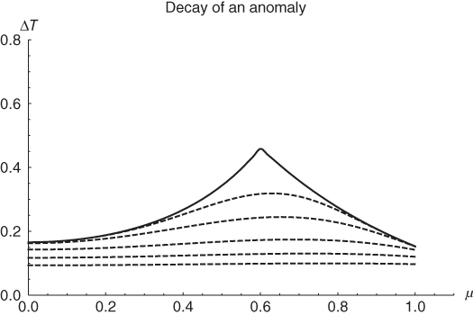
Figure 6.2 Decay of a symmetric (between the hemispheres) initial distribution (solid line) after times 0.25 , 0.5
, 0.5 , 0.75
 and
and  (dashed lines). The model parameters are as earlier and the sum is truncated at
  . The steady-state response has a discontinuous derivative at the ring's latitude. Its Fourier–Legendre series is very slowly converging, and this indicates that much power resides in higher-mode indices. These modes decay quickly leaving behind a smoother latitudinal profile as the temperature relaxes toward the old steady-state solution (zero here).
6.2.1 Decay of an Arbitrary Anomaly
An arbitrary distribution of thermal anomaly will decay in time according to a superposition of the modes just discussed. For example, an initial distribution of anomaly (departure from equilibrium) whose shape is ![]() will decay according to
will decay according to

For example, consider an initial shape rendered by a steady ring of heat source (Chapter 5) at a specific latitude as given by (5.11) and shown in Figure 5.11. The solid line in Figure 6.2 shows such a steady-state anomaly located at ![]() (37
(37![]() N). If suddenly the heat source is switched off, the distribution will decay according to (6.7). The figure shows stages of the decay at 0.25
N). If suddenly the heat source is switched off, the distribution will decay according to (6.7). The figure shows stages of the decay at 0.25![]() , 0.5
, 0.5![]() , 0.75
, 0.75![]() , and 1.00
, and 1.00![]() . We see that the higher modes, those rendering the cusp-like peak, are lost quickly leaving behind only the smoother long-lived modes.
. We see that the higher modes, those rendering the cusp-like peak, are lost quickly leaving behind only the smoother long-lived modes.
6.3 Seasonal Cycle on a Homogeneous Planet
We can begin the study of the seasonal cycle by placing the solar heating distribution as a forcing on the right-hand side of the energy-balance equation. The heating distribution can be written for a circular orbit as follows:
where ![]() , and
, and ![]() (see Figure 6.3). The subscripts denote the Legendre index first, then seasonal time harmonic second. A derivation for this heating distribution function is sketched in the appendix to this chapter. But for now we can observe some important properties. The mean annual version can be quickly recovered by averaging from 0 to 1 year in
(see Figure 6.3). The subscripts denote the Legendre index first, then seasonal time harmonic second. A derivation for this heating distribution function is sketched in the appendix to this chapter. But for now we can observe some important properties. The mean annual version can be quickly recovered by averaging from 0 to 1 year in ![]() ,
,
which is the formula used earlier in Chapter 5. The main part of the seasonal cycle is carried by the coefficient of the ![]() term. Note that it is antisymmetric between the hemispheres (recall the identity
term. Note that it is antisymmetric between the hemispheres (recall the identity ![]() ). The seasonal forcing is largest near the poles (
). The seasonal forcing is largest near the poles (![]() ). Another interesting feature captured by this representation is that along the equator (
). Another interesting feature captured by this representation is that along the equator (![]() ) there are two maxima (see Figure 6.3). This is the effect of the Sun crossing the equator twice each year at the equinoxes. Table A.6.1 shows the coefficients for some higher terms in the expansion for the present elliptical orbit of the Earth. Figure 6.4 shows the seasonal insolation when only modes 0, 1, and 2 are included. This figure indicates that retention of only these three modes captures the most important features of the insolation. Figure 6.5 shows how in the tropics there are two peaks as one passes through the year. The figure shows that for
) there are two maxima (see Figure 6.3). This is the effect of the Sun crossing the equator twice each year at the equinoxes. Table A.6.1 shows the coefficients for some higher terms in the expansion for the present elliptical orbit of the Earth. Figure 6.4 shows the seasonal insolation when only modes 0, 1, and 2 are included. This figure indicates that retention of only these three modes captures the most important features of the insolation. Figure 6.5 shows how in the tropics there are two peaks as one passes through the year. The figure shows that for ![]() the semiannual harmonic is strong. These three modes are able even to capture the passage of the Sun over the equator twice per year. Away from the equator, the seasonal harmonic dominates. Figure 6.6 shows latitudinal time sections of the forcing. The dashed lines show the forcing for zero eccentricity.
the semiannual harmonic is strong. These three modes are able even to capture the passage of the Sun over the equator twice per year. Away from the equator, the seasonal harmonic dominates. Figure 6.6 shows latitudinal time sections of the forcing. The dashed lines show the forcing for zero eccentricity.
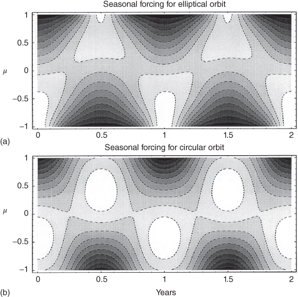
Figure 6.3 Contour diagrams of the seasonal forcing  or insolation. The vertical axis is cosine of colatitude,
  ; the horizontal axis is time,
  in years and
  corresponds to summer solstice for the Northern Hemisphere. The units of the contour plot is for the present elliptical orbit forcing through the Legendre mode 4 and time harmonic 2. The seasonal cycle of
  for the present elliptical orbit with eccentricity 0.016 (a) and the seasonal cycle for the same heating, but for a circular orbit (b). The value of time equal to zero in the Northern Hemisphere winter solstice.
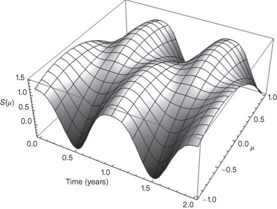
Figure 6.4 Seasonal cycle of  for the present orbital obliquity
  when only the Legendre modes 0, 1, and 2 are retained along with mean annual, annual harmonic, and semiannual harmonic. The time span is over 2 years in units of years with the origin at northern winter solstice. The latitudinal coordinate
  runs from the South pole (
 ) to the North Pole (
 ). The semiannual harmonic captures the passage of the Sun over the equator twice a year in this image.

Figure 6.5 Seasonal cycle of  in the tropics (
 ) for the present orbital obliquity
  when only the Legendre modes 0, 1, and 2 are retained along with mean annual, annual harmonic, and semiannual harmonic. This graphic shows the tropical variation with two maxima per year caused by the
  term. Note the change in vertical scale from the previous figure. The time span is over 2 years in units of years with the origin at northern winter solstice. Note that the details of polar day and night are missed in this truncation, but the semiannual harmonic captures the passage of the Sun over the equator twice a year.
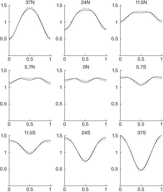
Figure 6.6 This figure illustrates the effect of eccentricity on the seasonal cycle of zonal average temperatures for an all-land planet. Shown is the modeled seasonal cycle (retaining Legendre modes 0, 1, and 2) of temperatures for the bare planet for present orbital parameters (solid curves) at selected latitudes:  0.6 (36.9N/S),
  0.4 (23.6N/S),
  0.2 (11.5N/S),
  0.1 (5.7N/S), and 0 (Equator). The dashed curves are for the corresponding circular orbit (
 ).
).
We can express the seasonal dependence of insolation as

If we take the coalbedo, diffusion coefficient, and heat capacity to be constants independent of season and latitude, we can write equations for the mode responses:

where ![]() is the constant coalbedo. To simplify the algebra. we employ complex notation (superscript
is the constant coalbedo. To simplify the algebra. we employ complex notation (superscript ![]() indicates a complex variable) and the complex Fourier series:
indicates a complex variable) and the complex Fourier series:

Inserting this into the governing mode equations:

To recover the physical mode amplitudes,
whereas the phase lag behind the forcing is

The complex ![]() are related to the real Fourier coefficients as follows:
are related to the real Fourier coefficients as follows:
After a time (![]() ), the transients die out and we are left with the repeating steady-state solutions. First, consider the time-independent parts:
), the transients die out and we are left with the repeating steady-state solutions. First, consider the time-independent parts:


Next, consider the seasonal harmonic terms:


and finally, the semiannual terms:


In each case, we can compute the amplitude

with phase lag

It is interesting to evaluate these quantities for the all-land planet. Using typical values of the parameters, ![]() W m
W m![]() ,
, ![]() W (m
W (m![]() K
K![]() ),
), ![]() ,
, ![]() , we find
, we find ![]() C,
C, ![]() K,
K, ![]() days,
days, ![]() K,
K, ![]() K,
K, ![]() days. While the phase lag is approximately correct for an all-land planet, the amplitude of both harmonics is larger than observed values for the Northern Hemisphere by a factor of about 4 (Northern Hemisphere zonal averages). These large amplitudes are due to the absence of ocean surface in the zonal averages. In the Northern Hemisphere, the land fraction is about 60% and in the Southern Hemisphere, the fraction is 80%. We will attempt to remedy this situation in Chapter 8 by introducing land–sea geography. Figure 6.7 shows the forcing for a circular orbit and the response superimposed in solid line contours. Note the lag of about a tenth of a year in the response. There is also a displacement poleward of the maximum response from the heating. Figure 6.8 indicates the response through time at some selected latitudes, this time including the effects of the eccentric orbit.
days. While the phase lag is approximately correct for an all-land planet, the amplitude of both harmonics is larger than observed values for the Northern Hemisphere by a factor of about 4 (Northern Hemisphere zonal averages). These large amplitudes are due to the absence of ocean surface in the zonal averages. In the Northern Hemisphere, the land fraction is about 60% and in the Southern Hemisphere, the fraction is 80%. We will attempt to remedy this situation in Chapter 8 by introducing land–sea geography. Figure 6.7 shows the forcing for a circular orbit and the response superimposed in solid line contours. Note the lag of about a tenth of a year in the response. There is also a displacement poleward of the maximum response from the heating. Figure 6.8 indicates the response through time at some selected latitudes, this time including the effects of the eccentric orbit.
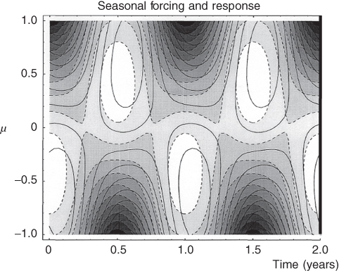
Figure 6.7 Illustration of the lag of zonal-average seasonal temperatures behind the forcing for the all-land planet. Shown is a contour plot (solid contours) of seasonal temperature response for the circular orbit insolation in dashed contours superimposed on the forcing to show the lag between heating and response. For a mixed-layer all-ocean planet where the response time is several years, the lag will be close to  radians or 0.25 year.

Figure 6.8 EBM solutions for the seasonal cycle of  for the all-land planet with present orbital parameters at selected latitudes:
  0.6 (36.9N/S),
  0.4 (23.6N/S),
  0.2 (11.5N/S),
  0.1 (5.7N/S) and 0 (equator).
6.4 Spread of Diffused Heat
Since EBMs make use of diffusion as a mechanism to transport heat poleward in the atmosphere/ocean system, it is useful to see how diffusion is related to random walk processes. Random walk means that the progress (root mean square average distance from the point of origination) of a passive scalar is the sum of a large number of steps. Let ![]() be the random variable denoting the displacement after
be the random variable denoting the displacement after ![]() steps. We can write
steps. We can write

The mean over an ensemble of such random walks is 0, because we assume the individual steps have mean 0, that is,

The variance of ![]() can be calculated if all the
can be calculated if all the ![]() are uncorrelated and have equal variance:
are uncorrelated and have equal variance:
The standard deviation of ![]() is proportional to the square root of the number of steps.
is proportional to the square root of the number of steps.
Now consider the one-dimensional damped diffusion equation

It is convenient to solve this equation with Fourier transforms. ![]() can be represented as follows:
can be represented as follows:

We can write the second spatial partial derivative as follows:

The inverse Fourier transform is

We can insert the other terms.

The integrand must vanish for every wave number.

The solution to this first-order homogeneous linear equation for wave number ![]() is
is
If the initial distribution is peaked at ![]() , that is,
, that is, ![]() , then
, then ![]() , a constant. The inverse Fourier transformation
, a constant. The inverse Fourier transformation

gives (from tables or MATHEMATIC A)

where we have used the now familiar length scale ![]() and
and ![]() to make the notation more compact and to see the variables
to make the notation more compact and to see the variables ![]() and
and ![]() proportional to their natural scales,
proportional to their natural scales, ![]() and
and ![]() . We see that except for the overall damping factor
. We see that except for the overall damping factor ![]() , the solution spreads like a bell-shaped curve with standard deviation
, the solution spreads like a bell-shaped curve with standard deviation
The interpretation is that heat spreads symmetrically away from a point-concentrated initial anomaly a distance that is comparable to the damped diffusive length scale ![]() in about one characteristic time
in about one characteristic time ![]() . This is shown in Figure 6.9, wherein the spatial units are proportional to
. This is shown in Figure 6.9, wherein the spatial units are proportional to ![]() and temporal units are proportional to
and temporal units are proportional to ![]() .
.
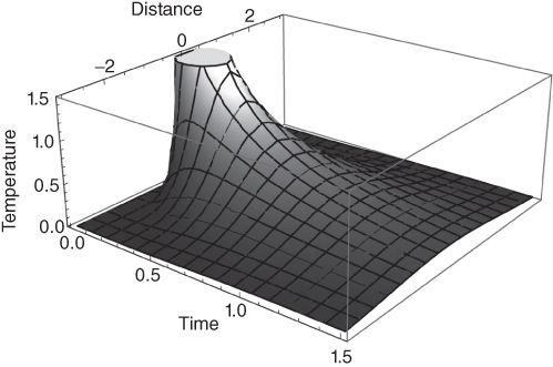
Figure 6.9 Temporal evolution of a point pulse of heat at the origin at time equal to 0. Horizontal distance in units of  , temporal span in units of
  .
.
6.4.1 Evolution on a Plane
This section generalizes the treatment to two horizontal dimensions on the infinite ![]() –
–![]() plane. We begin by including diffusion in two Cartesian dimensions:
plane. We begin by including diffusion in two Cartesian dimensions:

This time we use the two-dimensional Fourier transform pair (in the two spatial dimensions):

where the two-dimensional vectors ![]() and
and ![]() have been introduced. Following the steps from the subSection 6.4, we find
have been introduced. Following the steps from the subSection 6.4, we find

where ![]() , and the integration limits
, and the integration limits ![]() have been suppressed. We proceed by using polar coordinates in the
have been suppressed. We proceed by using polar coordinates in the ![]() plane. We write
plane. We write ![]() where
where ![]() is the angle between the vectors
is the angle between the vectors ![]() and
and ![]() , and
, and ![]() .
.

We proceed by considering first the portion of the double integral into its ![]() part (enclosed in parentheses): This angular integral is well known (it is a special case,
part (enclosed in parentheses): This angular integral is well known (it is a special case, ![]() , of Bessel's integral (see Whittacker and Watson, 1962 p. 362; or other books on mathematical physics)):
, of Bessel's integral (see Whittacker and Watson, 1962 p. 362; or other books on mathematical physics)):

where ![]() is the Bessel function. The resulting integral can also be solved (e.g., MATHEMATICA), yielding the rather unsurprising answer:
is the Bessel function. The resulting integral can also be solved (e.g., MATHEMATICA), yielding the rather unsurprising answer:

Note that in this compact form ![]() is expressed proportional to the damped diffusion length scale
is expressed proportional to the damped diffusion length scale ![]() and
and ![]() is always found proportional to the global timescale
is always found proportional to the global timescale ![]() . We have found exactly what we found in one dimension: a delta function point expanding into a 2-D Gaussian shape, further expanding its disk width in a time
. We have found exactly what we found in one dimension: a delta function point expanding into a 2-D Gaussian shape, further expanding its disk width in a time ![]() that is about
that is about ![]() in radius. The volume under the Gaussian surface also diminishes by the factor
in radius. The volume under the Gaussian surface also diminishes by the factor ![]() owing to the damping from infrared radiation to space.
owing to the damping from infrared radiation to space.
6.5 Random Winds and Diffusion
Next consider the one-dimensional energy-balance equation in which heat is advected by a wind field that for simplicity has no ![]() -dependence.
-dependence.

Once again, look at the component of the wave number ![]()

This is a first-order linear equation and can be solved using the usual integrating factor:

Let ![]() be a stationary random function of time. The ensemble average of a random quantity is denoted by
be a stationary random function of time. The ensemble average of a random quantity is denoted by ![]() . Let the ensemble average vanish; stationarity demands that
. Let the ensemble average vanish; stationarity demands that ![]() with
with ![]() . This means that
. This means that ![]() will have mean zero and be stationary as well. Finally, we assume that
will have mean zero and be stationary as well. Finally, we assume that ![]() is a Gaussian random field. In other words, our wind field is similar to a random eddy field that carries heat one way or another depending on the vagaries of such a wind field. Note, however, that we have not permitted the wind to be a function of position. This makes our wind field a rather peculiar one: at a point in time it is everywhere pointed in the same direction, until the next instant, when it suddenly switches direction and magnitude the same everywhere. The case of the wind field that is variable in space as well as time is more difficult to solve. Rather than going into the complexities involved in that, we proceed with what we have.
is a Gaussian random field. In other words, our wind field is similar to a random eddy field that carries heat one way or another depending on the vagaries of such a wind field. Note, however, that we have not permitted the wind to be a function of position. This makes our wind field a rather peculiar one: at a point in time it is everywhere pointed in the same direction, until the next instant, when it suddenly switches direction and magnitude the same everywhere. The case of the wind field that is variable in space as well as time is more difficult to solve. Rather than going into the complexities involved in that, we proceed with what we have.
Consider the series expansion of the second exponential factor, ![]() .
.
The first three terms are

The second term vanishes because ![]() . In fact, all the odd powered terms vanish.a We turn to the third term after running the integrals from time
. In fact, all the odd powered terms vanish.a We turn to the third term after running the integrals from time ![]() to
to ![]() instead of 0 to
instead of 0 to ![]() . This symmetry helps in analyzing the result.
. This symmetry helps in analyzing the result.

Figure 6.10 Geometry for a two-dimensional integral over a lag covariance function for a stationary process:  . Since
  only depends on
  , we can find the integral by summing the diagonal infinitesimal strip whose width is
  . The value of
  in the lower-right corner is
  and its value in the upper-left corner is
  . The quantity to be summed is the length of the diagonal strip (
 ) times
  . The integral becomes
  . (Redrawn from original figures in Papoulis (1984).)

The double integral can be computed by a transformation of variables from ![]() to a one-dimensional integral. Referring to Figure 6.10, as the integrand only depends on
to a one-dimensional integral. Referring to Figure 6.10, as the integrand only depends on ![]() , the integration is best done by summing slabs that are at a 45
, the integration is best done by summing slabs that are at a 45![]() angle (along which
angle (along which ![]() ) to the horizontal. The length of the slab can be found from the hypotenuse of the right isosceles triangle whose lower edge has length
) to the horizontal. The length of the slab can be found from the hypotenuse of the right isosceles triangle whose lower edge has length ![]() . We can show this last by noting that the same side has length
. We can show this last by noting that the same side has length ![]() where
where ![]() is evaluated at the point the hypotenuse intersects the line
is evaluated at the point the hypotenuse intersects the line ![]() . At that point,
. At that point, ![]() , or
, or ![]() . Using
. Using ![]() we finally arrive at the width of thelower side of the triangle to be
we finally arrive at the width of thelower side of the triangle to be ![]() . The length of the slab is
. The length of the slab is ![]() . The width of the slab is
. The width of the slab is ![]() ; the two square roots cancel to leave us with
; the two square roots cancel to leave us with

where ![]() is the autocorrelation function for the magnitude of the lag
is the autocorrelation function for the magnitude of the lag ![]() . Note that
. Note that ![]() and
and ![]() is the variance of the velocity field. We specify that the integration time
is the variance of the velocity field. We specify that the integration time ![]() is very long compared to the autocorrelation time
is very long compared to the autocorrelation time ![]() that we take to be
that we take to be ![]() in Figure 6.11. This means that the kernel (nearly an isosceles triangle of base width 2
in Figure 6.11. This means that the kernel (nearly an isosceles triangle of base width 2![]() and height unity) of the integral is concentrated near
and height unity) of the integral is concentrated near ![]() and the integral is
and the integral is ![]() , which is
, which is
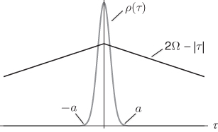
Figure 6.11 Depiction of how a short autocorrelation time leads to an estimate of a double integral related to second moments.
(Redrawn from original figures in Papoulis (1984).)
After replacing ![]() by
by ![]() to regain the original notation, we can now identify
to regain the original notation, we can now identify
which gives us a handy formula for the diffusion coefficient in terms of the variance of the wind speed and its autocorrelation time. The last expression is reminiscent of the form of (6.36). Note that the units of ![]() are (length)
are (length)![]() (time)
(time)![]() , when the diffusion equation is set with the coefficient of
, when the diffusion equation is set with the coefficient of ![]() set to unity. When the approximations above are valid, we can think of diffusion equations as being the equations describing the ensemble averages of (damped) random walk equations. Basically, the approximation is that the winds are white noise (
set to unity. When the approximations above are valid, we can think of diffusion equations as being the equations describing the ensemble averages of (damped) random walk equations. Basically, the approximation is that the winds are white noise (![]() days) compared to our averaging times. All timescales, including relaxation time of a column of air (
days) compared to our averaging times. All timescales, including relaxation time of a column of air (![]() 30 days), and forcing functions such as the seasonal cycle (few months), must be long compared to the weather–noise timescale (few days). This suggests the following:
30 days), and forcing functions such as the seasonal cycle (few months), must be long compared to the weather–noise timescale (few days). This suggests the following:

When this approximation is valid, we can safely think of the EBCM equation as an equation for the ensemble average of ![]() . Note that there is a residual whose ensemble average is zero. Later, we will use this residual as a noise driver of climate fluctuations.
. Note that there is a residual whose ensemble average is zero. Later, we will use this residual as a noise driver of climate fluctuations.
6.6 Numerical Methods
6.6.1 Explicit Finite Difference Method
We start with the energy-balance equation:

where

The coefficient in (6.51) was constructed by multiplying numerator and denominator by ![]() , then using
, then using ![]() and
and ![]() . We start with a grid from
. We start with a grid from ![]() 1 to 1, divided into
1 to 1, divided into ![]() equal segments. More details on the grid are presented in the following. The centered finite difference form for the derivative is
equal segments. More details on the grid are presented in the following. The centered finite difference form for the derivative is

The derivative of ![]() is then
is then

where
To step forward in time, we have the following algorithm (in the explicit finite difference case):

where the important parameter ![]() is given by
is given by
Next, we must make sure our solution enforces the Neumann boundary conditions, implying that no net heat flux enters the infinitesimal latitude circles surrounding the poles:

The fact that the time-dependent version of the equation has a regular singular point at the pole poses a problem because as noted earlier, small numerical errors will lead to erroneous encroachment by the irregular solutions (![]() ). This does not turn out to be a serious problem as we will see. The most straightforward way of representing the equation in finite difference form is to break the interval
). This does not turn out to be a serious problem as we will see. The most straightforward way of representing the equation in finite difference form is to break the interval ![]() into
into ![]() intervals,
intervals, ![]() . Similarly, the time is discretized in steps of
. Similarly, the time is discretized in steps of ![]() .
.
Deferring discussion of the boundary points, we see that the term on the left is the value of ![]() at time
at time ![]() , while all the terms on the right are to be evaluated at the previous time
, while all the terms on the right are to be evaluated at the previous time ![]() . This is very convenient because we presumably have knowledge of the field at time
. This is very convenient because we presumably have knowledge of the field at time ![]() . For example, if we start at time
. For example, if we start at time ![]() , we know the initial profile of the field. This process allows us to evaluate it at
, we know the initial profile of the field. This process allows us to evaluate it at ![]() and so on. Such an algorithm is very appealing intuitively as it feels like we are solving the equation just as nature does it. Note that there is a problem at the end points for the reason that when
and so on. Such an algorithm is very appealing intuitively as it feels like we are solving the equation just as nature does it. Note that there is a problem at the end points for the reason that when ![]() , the RHS contains the value
, the RHS contains the value ![]() and when
and when ![]() , it contains the value
, it contains the value ![]() . Hence, we must use the aforementioned algorithm only for
. Hence, we must use the aforementioned algorithm only for ![]() . Had the boundary conditions been of the Dirichlet type where the values of the field are specified at the boundaries, we could merely specify the values of
. Had the boundary conditions been of the Dirichlet type where the values of the field are specified at the boundaries, we could merely specify the values of ![]() and
and ![]() .
.
Enforcing the Neumann boundary conditions is a little tricky as the straightforward implementation of the thinking above leads to ![]() and
and ![]() . We can get around this by using a centered difference of width
. We can get around this by using a centered difference of width ![]() for these points. We introduce fictitious points just outside the range,
for these points. We introduce fictitious points just outside the range, ![]() , and
, and ![]() . Then the boundary conditions read as follows:
. Then the boundary conditions read as follows:

We compute the outside points using the explicit algorithm, but then force ![]() to equal the lower outside value
to equal the lower outside value ![]() and likewise
and likewise ![]() is forced to be
is forced to be ![]() .
.
The curves in Figure 6.12 show an example of implementation of this kind of algorithm for ![]() , where we have modified the definition of the parameter
, where we have modified the definition of the parameter ![]() to include
to include ![]() , that is,
, that is, ![]() , thereby allowing the stability parameter to be a function of latitude. The forcing is
, thereby allowing the stability parameter to be a function of latitude. The forcing is ![]() . The initial condition for the integration is
. The initial condition for the integration is ![]() C. There are 20 intervals in
C. There are 20 intervals in ![]() from pole to pole, and the time step is
from pole to pole, and the time step is ![]() of the relaxation time
of the relaxation time ![]() . The figure shows a sequence of profiles after 10, 20, 40, 80, 160, 320, and 640 time steps. The last is nearly indistinguishable from the 320 time-step case. The solutions in this case are smooth and stable after integration to 3.20 relaxation times. Advancement to 3000 steps (30 relaxation times) indicates no change. We infer stability of the solution.
. The figure shows a sequence of profiles after 10, 20, 40, 80, 160, 320, and 640 time steps. The last is nearly indistinguishable from the 320 time-step case. The solutions in this case are smooth and stable after integration to 3.20 relaxation times. Advancement to 3000 steps (30 relaxation times) indicates no change. We infer stability of the solution.
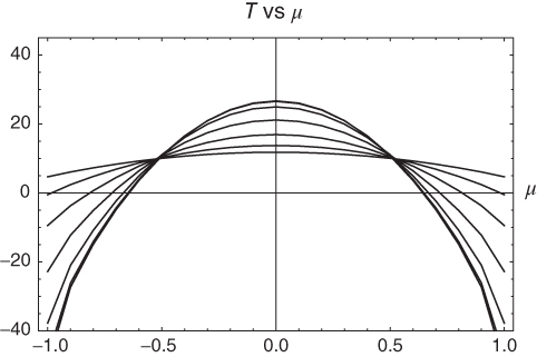
Figure 6.12 Sequence of the evolution toward steady state where the forcing is the usual  . The initial condition is flat with
  C. The time step is 0.05, which is 1/20 of the relaxation time,
  . The individual graphs are at
  , and 640 steps. In this case,
  W m
W m C)
C) . An additional run (not shown) of length 3000 steps showed no change.
If we increase the time step by a factor of 10 to 0.1![]() , we run into trouble. This case is shown in Figure 6.13 starting from the same initial condition. The stability parameter
, we run into trouble. This case is shown in Figure 6.13 starting from the same initial condition. The stability parameter ![]() increases to 3.20. In the integration, everything goes well until time step 400 in which a small ripple occurs at the equator. By time step 425, the instability is full blown and propagating from the equator toward the poles. The reason for this peculiar behavior is that the explicit method is unstable when the time steps are too large compared to the spatial increment. For the diffusion equation, the condition can be made quantitative: the solution will be unstable if
increases to 3.20. In the integration, everything goes well until time step 400 in which a small ripple occurs at the equator. By time step 425, the instability is full blown and propagating from the equator toward the poles. The reason for this peculiar behavior is that the explicit method is unstable when the time steps are too large compared to the spatial increment. For the diffusion equation, the condition can be made quantitative: the solution will be unstable if ![]() . Since
. Since ![]() is largest at the equator, the instability breaks out there first as indicated in the figure. The physical interpretation of the instability is that for diffusion or random walk processes, information propagates an rms distance
is largest at the equator, the instability breaks out there first as indicated in the figure. The physical interpretation of the instability is that for diffusion or random walk processes, information propagates an rms distance ![]() . Turning this around, we have
. Turning this around, we have ![]() ; if
; if ![]() in the numerical integration is larger than the time for propagation of information in the continuous exact solution, we can expect instability of the numerical procedure. A similar limitation occurs in the integration of wavelike (hyperbolic) equations with wave motion entering as the propagation mechanism (
in the numerical integration is larger than the time for propagation of information in the continuous exact solution, we can expect instability of the numerical procedure. A similar limitation occurs in the integration of wavelike (hyperbolic) equations with wave motion entering as the propagation mechanism (![]() ,
, ![]() = wave speed).
= wave speed).

Figure 6.13 The smooth line represents the approximate solution after 300 time steps where the approximate solution seems to have settled down to the correct answer. But if the integration continues to 425 steps, one encounters the spiky line indicating numerical instability. In this case,  W m
W m C)
C) .
.
The finite difference algorithm as noted above in (6.56) is not the only one that is accurate with errors of order (![]() ). The next subsection considers some alternatives that have different numerical stability properties.
). The next subsection considers some alternatives that have different numerical stability properties.
6.6.2 Semi-Implicit Method
An intermediate method is often used in practice. It is simply the weighted average of the explicit and implicit algorithms:

with ![]() .
.
One has to gather the coefficients of ![]() and place them onto the left-hand side. The coefficient matrix has to be inverted to obtain
and place them onto the left-hand side. The coefficient matrix has to be inverted to obtain ![]() . The result is
. The result is

where ![]() is a large matrix with
is a large matrix with ![]() and
and ![]() spatial indices. The matrix has to be inverted to find the next time-step values as a function latitude as indicated by the index
spatial indices. The matrix has to be inverted to find the next time-step values as a function latitude as indicated by the index ![]() :
: ![]() . Fortunately, the matrix
. Fortunately, the matrix ![]() is usually sparse (most entries are zero), and very fast algorithms are available. A special case that is commonly used is for
is usually sparse (most entries are zero), and very fast algorithms are available. A special case that is commonly used is for ![]() , which is called the Crank–Nicolson scheme. Stability properties can be found in books on numerical analysis, but experience shows that use of this method allows larger time steps before instability sets in. Semi-implicit algorithms are commonly used in numerical solution of general circulation models.
, which is called the Crank–Nicolson scheme. Stability properties can be found in books on numerical analysis, but experience shows that use of this method allows larger time steps before instability sets in. Semi-implicit algorithms are commonly used in numerical solution of general circulation models.
In the finite difference solution to more complicated models treating dynamics of the flows as well as radiation, and so on, it is found to be advantageous to treat some terms on the RHS of the equation with one semi-implicit weighting and other terms with different weightings. These are called splitting methods. Again, they are commonly used in numerical solutions of climate models.
6.7 Spectral Methods
6.7.1 Galerkin or Spectral Method
An alternative to the finite difference methods is to write an approximate solution to the field as a series of (usually) orthogonal functions

where ![]() is some finite cutoff to the series. A rather obvious choice for the
is some finite cutoff to the series. A rather obvious choice for the ![]() for this class of problems is the Legendre polynomials,
for this class of problems is the Legendre polynomials, ![]() . In the present case, this renders the problem trivial as the
. In the present case, this renders the problem trivial as the ![]() are the eigenfunctions of
are the eigenfunctions of ![]() . The problem becomes nontrivial if the diffusion coefficient depends on
. The problem becomes nontrivial if the diffusion coefficient depends on ![]() . Such an EBM may be written as
. Such an EBM may be written as

with the usual Neumann boundary conditions at the poles. If ![]() is inserted and each side is multiplied by
is inserted and each side is multiplied by ![]() and integrated from pole to pole with respect to
and integrated from pole to pole with respect to ![]() , we obtain
, we obtain

where

Now the problem has been reduced to a set of ![]() first-order coupled ordinary differential equations for the time-dependent coefficients
first-order coupled ordinary differential equations for the time-dependent coefficients ![]() . The coupling matrix is symmetric, hence in this case we can even find its eigenvectors and conduct a stability analysis. From discussions earlier in this chapter, it is easy to relate the eigenvalues to relaxation times for the eigenmodes of the problem. The numerical integration will be unstable if the time constant for the highest eigenmode retained (
. The coupling matrix is symmetric, hence in this case we can even find its eigenvectors and conduct a stability analysis. From discussions earlier in this chapter, it is easy to relate the eigenvalues to relaxation times for the eigenmodes of the problem. The numerical integration will be unstable if the time constant for the highest eigenmode retained (![]() th) is shorter than the time step employed in the time-stepping algorithm. In other words, the criterion encountered in the explicit scheme comes up again unless special precautions are taken.
th) is shorter than the time step employed in the time-stepping algorithm. In other words, the criterion encountered in the explicit scheme comes up again unless special precautions are taken.
Other basis sets are possible besides the Legendre polynomials. For example, one might try a Fourier series

This choice is equivalent to the use of Chebyshev polynomials. This method is successful in the present one-dimensional case but requires considerable work and extra discussion when applied to the case of two horizontal dimensions. One advantage is that transformations from grid points to components ![]() and vice-versa can be accomplished via fast Fourier transform.
and vice-versa can be accomplished via fast Fourier transform.
6.7.2 Pseudospectral Method
A complication arises in the spectral method if one of the coefficients is space dependent, for example, ![]() . Then,
. Then,

with

and

where

and the ![]() are known as interaction coefficients. They can be tabulated or generated from recurrence relations. It is important to notice how many are necessary in a high-resolution simulation. For example, in a GCM simulation the truncation level might be 15 or 42 typically. This means there are 3375 or 74 088 coefficients that have to be stored in a lookup table. Some storage savings can be gained by noting that most of the interaction coefficients are 0. However, when the problem is elevated to two dimensions on the sphere, it becomes truly formidable. One way to get around it is to use a so-called pseudospectral method.
are known as interaction coefficients. They can be tabulated or generated from recurrence relations. It is important to notice how many are necessary in a high-resolution simulation. For example, in a GCM simulation the truncation level might be 15 or 42 typically. This means there are 3375 or 74 088 coefficients that have to be stored in a lookup table. Some storage savings can be gained by noting that most of the interaction coefficients are 0. However, when the problem is elevated to two dimensions on the sphere, it becomes truly formidable. One way to get around it is to use a so-called pseudospectral method.
In the pseudospectral method, we transform back and forth between a grid point representation and the spectral representation. The grid point representation for the sphere involves use of the Gaussian quadrature method of numerically estimating integrals. An integral may be estimated by the sum

where the ![]() are weights associated with each term and the
are weights associated with each term and the ![]() are unequally spaced but specified points along the axis. The
are unequally spaced but specified points along the axis. The ![]() and
and ![]() are optimal for a given level
are optimal for a given level ![]() . Gaussian integrationb of order
. Gaussian integrationb of order ![]() has the property that it integrates a
has the property that it integrates a ![]() degree polynomial exactly. The abscissas
degree polynomial exactly. The abscissas ![]() are the
are the ![]() zero of
zero of ![]() and the weights
and the weights ![]() are
are ![]() . As an example, Figure 6.14 shows a plot of
. As an example, Figure 6.14 shows a plot of ![]() (solid gray line) along with a plot of
(solid gray line) along with a plot of ![]() (black line) with heavy points on the dashed line corresponding to the value of the weights at the roots
(black line) with heavy points on the dashed line corresponding to the value of the weights at the roots ![]() of
of ![]() . Next, the quantities
. Next, the quantities ![]() and
and ![]() are calculated by
are calculated by


Figure 6.14 Plot of  (solid gray curve) with zeros at
  . Also a plot of
  (heavy black U-shaped curve) with vertical thin black lines corresponding to the value of the weights at the roots
  of
of  . The ordinate values of the intersections are the weights. The graph is only shown for
  , as all the functions are even.
The next time step may now be evaluated:

where the ratio on the LHS stands for time advancement by some ODE algorithm such as Runge–Kutta. When the new set ![]() are computed, we can reevaluate
are computed, we can reevaluate ![]() by
by

The procedure delineated in (6.76)–(6.79) can be repeated as many times as necessary as long as the employed ODE algorithm is stable.
Studies have shown that the pseudo-spectral method pays over the interaction coefficient method when the number of stored coefficients exceeds a few tens of thousands. Since this is rather quickly exceeded in GCM calculations, the pseudospectral method is commonly used in numerical simulations.
6.8 Summary
This chapter has introduced time into the energy balance models. The first result is that for the linear zonally symmetric models, we find that if a climate is perturbed from equilibrium and then released, it relaxes back to its steady-state solution. The relaxation can be characterized as a sum of contributions from relaxation modes, each having an exponential decay with large scales having longer relaxation times than smaller ones. The zonally symmetric planet can also be solved for its seasonal cycle. It is remarkable that the solar insolation can be represented for many purposes as a sum of terms involving only the Legendre modes 0, 1, and 2. The largest part of the circular orbital insolation is controlled by Legendre mode of index 1, which is antisymmetric on the globe and driven by a single annual cycle sinusoid in time. The Legendre mode of index 2 also has a non-negligible contribution in the semiannual cycle representing the passage of the Sun over the equator twice per year. These simple facts allow the seasonal cycle to be solved for this configuration. We can readily study the major effects on insolation of changing orbital parameters. The amplitude of the annual cycle is much too large if the zonally symmetric planet is considered to be all-land and too smallif all-ocean. We postpone the study of land–sea distribution until Chapter 8.
Next in the chapter was a study of how a patch of heat deposited in a small area spreads laterally to larger circular areas in a time roughly that of the characteristic time of the global model, ![]() to a radius of the characteristic length
to a radius of the characteristic length ![]() . The spread has an exponentially damped (time constant
. The spread has an exponentially damped (time constant ![]() ) Gaussian shape with standard deviation proportional to
) Gaussian shape with standard deviation proportional to ![]() . It was also shown that if the diffusion term is replaced by a random-wind advection term, the ensemble result will be the same as diffusion. If the autocorrelation time of the velocity field is short compared to other times, such as
. It was also shown that if the diffusion term is replaced by a random-wind advection term, the ensemble result will be the same as diffusion. If the autocorrelation time of the velocity field is short compared to other times, such as ![]() , in the problem, then the ensemble average of this term is essentially the diffusion term. This is very close to the Brownian motion problem solved by Einstein in 1904.
, in the problem, then the ensemble average of this term is essentially the diffusion term. This is very close to the Brownian motion problem solved by Einstein in 1904.
The chapter concludes with a study of how 1-D EBMs can be solved by finite difference methods. In particular, an explicit problem is worked through in some detail with an illustration of how the procedure becomes unstable if the time step exceeds a certain threshold depending on the characteristic time and length scales of the EBM. Basically, the time step must be shorter than the spreading time across a grid box in the horizontal direction.
The appendix to the chapter provides some derivations of the orbital dependence of the insolation function.
6.8.1 Parameter Count
We have introduced the time dimension, which means we must now have an effective heat capacity that cannot be calculated from first principles. For the all-land planet and at frequencies around 1/year, our guess is to take it to be 1/2 the heat capacity of the air column's mass at constant pressure. This neglects the heat capacity of soil. We are also neglecting the topography, where atop mountains, the effective heat capacity might be less. For an all-ocean planet we take the effective heat capacity to be that of the ocean's mixed layer. It depends on position, especially latitude, but we take it to be constant. So for the latitude-only model we have introduced one new parameter, but we have learned a lot about how the seasonal cycle works for a uniform planet.
Notes for Further Reading
Papoulis (1984) is an excellent book on random processes and spectral analysis written mainly for electrical engineers. It is rather compact, but comprehensive. Numerical methods for partial differential equations are covered in Ames (1992) and Fletcher (1991). Multigrid methods for solving partial differential equations are covered in Hackbusch (1980) and Briggs et al. (2000) and applied to EBMs by Bowman and Huang (1991), Huang and Bowman (1992), and Stevens and North (1996). Mars has no ocean, so a constant heat capacity can be used on the (approximately) homogeneous planet. A one-dimensional model with a zonally symmetric seasonal cycle was used successfully by James and North (1982). Much more can be found about the Martian climate as well as the other planets in Ingersoll's recent book on planetary climates Ingersoll (2015). Planetary climates are covered at a higher level of physics by Pierrehumbert (2011).
Exercises
- 6.1 Given the time-dependent, one-dimensional energy balance model

where
 , and coalbedo
  are constants, derive the basic timescale and spatial scale of the model by nondimensionalizing the model.
 - 6.2 Consider the time-dependent, one-dimensional model of the previous exercise, where the parameters,
 , and
, and  are constants. Let the solution of the energy balance model be denoted as follows:
  . An external forcing is applied at time
  so that the temperature field is perturbed into the form
  . The external forcing disappears instantaneously (delta function in time). (a) Derive the governing equation for
  . (b) Solve the governing equation to obtain the solution for
  .
.
- 6.3 Consider next the same one-dimensional model as before with the same constant parameters. Let the solar distribution function be decomposed as follows:

where Re(
 ) denotes the real part of its argument. Solve the energy balance model for
  .
. - 6.4 Show that the solution of the one-dimensional damped diffusion equation

with the initial condition
 is given by
where
 and
and  .
. - 6.5 A semi-implicit algorithm for a time-dependent, one-dimensional energy balance model is given by

where

and
 and
and  denote a point in space and time, respectively. This equation can be rewritten as
Determine the matrices
 and
and  explicitly.
 - 6.6 Consider a time-dependent, one-dimensional energy balance model in the form

where
 represents the constant heat capacity and
  . Set up the solution procedure using the spectral method. Use the Legendre polynomials as basis functions.
 - 6.7 In Chapter 5, the insolation distribution function was determined by using spherical geometry. Consider the situation depicted in Figure 6.15. (a) Determine the normal vector at point
 and at point
  in terms of the longitude, latitude, and declination angle, and unit vectors i , j, and k. Then, calculate the cosine of the angle between the two vectors. (b) Determine the range of longitude for which the Sun is visible. (c) Based on your answers for (a) and (b), determine the total amount of insolation received at the surface when the solar constant is
  .
.
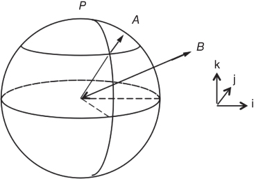
Figure 6.15 Diagram for Exercise 6.7.
6.9 Appendix to Chapter 6: Solar Heating Distribution
This chapter made use of the solar heating (insolation) function ![]() , which is the amount of radiant energy per unit time per unit surface area averaged through the day reaching the top of the atmosphere. In this appendix, we present a short derivation of this function, as its development into Legendre functions in latitude and sinusoids in time helps to understand the excitation of these modes in the response field under different orbital conditions. The appendix is organized as follows. First the derivation of
, which is the amount of radiant energy per unit time per unit surface area averaged through the day reaching the top of the atmosphere. In this appendix, we present a short derivation of this function, as its development into Legendre functions in latitude and sinusoids in time helps to understand the excitation of these modes in the response field under different orbital conditions. The appendix is organized as follows. First the derivation of ![]() is given, followed by a discussion of how the orbital elements enter the mode amplitudes. Figure 6.16 shows an octant of the Earth's surface with a given point
is given, followed by a discussion of how the orbital elements enter the mode amplitudes. Figure 6.16 shows an octant of the Earth's surface with a given point ![]() singled out for our attention. The North Pole lies in the
singled out for our attention. The North Pole lies in the ![]() direction, and hence the point
direction, and hence the point ![]() will rotate uniformly around the
will rotate uniformly around the ![]() -axis in the course of a day. As the day passes,
-axis in the course of a day. As the day passes, ![]() will vary linearly from 0 to
will vary linearly from 0 to ![]() . At a given time of day,
. At a given time of day, ![]() , the amount of solar power per unit area deposited at
, the amount of solar power per unit area deposited at ![]() is given by the solar constant
is given by the solar constant ![]() times the cosine of the angle between zenith direction
times the cosine of the angle between zenith direction ![]() and the line joining the Sun and the Earth
and the line joining the Sun and the Earth ![]() . In other words,
. In other words, ![]() . We define the solar vector
. We define the solar vector ![]() to lie in the
to lie in the ![]() plane. Using the Cartesian unit vectors
plane. Using the Cartesian unit vectors ![]() , and
, and ![]() , we may write
, we may write
where ![]() is the angle the solar vector makes with the equatorial plane (
is the angle the solar vector makes with the equatorial plane (![]() –
–![]() plane). Clearly,
plane). Clearly, ![]() depends on the time of the year. We readily compute
depends on the time of the year. We readily compute

Figure 6.16 An octant of the Earth's surface showing a unit vector toward the Sun  , lying in the
  plane. A given point on the Earth's surface is designated
  . The North Pole is along the
  -axis. The local time of day at point is proportional to
  . The declination
  is the angle the Sun makes with a perpendicular to the equatorial plane (the
  –
– plane here) for a given day of the year,
  . The declination depends on the tilt of the Earth's axis with respect to a perpendicular to the plane of the ecliptic (the obliquity) and the time of the year.
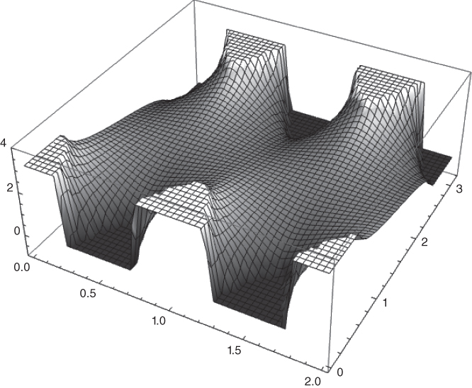
Figure 6.17 Half length of daylight in radians as a function of time of the year ( ) and the polar angle
  for obliquity
  and eccentricity
  . When the half day
  , it indicates perpetual daylight. The obliquity is chosen to be 35
 (as opposed to its present value of 23.47
 ) for illustration.

Figure 6.18 Graphic of the seasonal cycle of heating energy flux at the top of the atmosphere for a circular orbit and obliquity  as a function. The function is normalized by the total solar irradiance
  . (a) The three mode (
 ) insolation function. (b) The exact solution as described in Appendix A. A larger value of obliquity (
 ) is used to illustrate the polar day and night characteristics in the figure.
To obtain the diurnal average of the solar power at ![]() per unit area, we must integrate
per unit area, we must integrate ![]() through the daylight hours (the range of
through the daylight hours (the range of ![]() for which
for which ![]() ) and divide by the length of the whole day (
) and divide by the length of the whole day (![]() ). Dawn and dusk can be defined as
). Dawn and dusk can be defined as ![]() , the roots of
, the roots of ![]() .
.
The half day is shown in Figure 6.17. The formula can now be written for the solar power per unit area averaged through the day,
where ![]() differs slightly from the total solar irradiance (because it is not annualized). Because of the elliptical orbit,
differs slightly from the total solar irradiance (because it is not annualized). Because of the elliptical orbit,

where ![]() is the Earth–Sun distance at the given time of year and
is the Earth–Sun distance at the given time of year and ![]() is the annual average of
is the annual average of ![]() . Figure 6.18 shows the seasonal cycle of insolation function for a circular orbit.
. Figure 6.18 shows the seasonal cycle of insolation function for a circular orbit.
6.9.1 The Elliptical Orbit of the Earth
The Sun lies at the focus of an ellipse that constitutes the Earth's trajectory over the year (Figure 6.19). Using the Sun as the origin of a polar coordinate system with ![]() as polar angle in the ecliptic plane (celestial longitude), we can write
as polar angle in the ecliptic plane (celestial longitude), we can write

where ![]() is the eccentricity (presently
is the eccentricity (presently ![]() ),
),
and ![]() is very nearly the average of
is very nearly the average of ![]() (to fourth order in powers of
(to fourth order in powers of ![]() ). The value of
). The value of ![]() determines the time of year of the closest approach of the Earth to the Sun (perihelion). If we arbitrarily choose that
determines the time of year of the closest approach of the Earth to the Sun (perihelion). If we arbitrarily choose that ![]() at winter solstice (
at winter solstice (![]() December 22 in the present epoch), then at present
December 22 in the present epoch), then at present ![]() , as perihelion occurs at present within a few weeks of (Northern Hemisphere) winter solstice. However,
, as perihelion occurs at present within a few weeks of (Northern Hemisphere) winter solstice. However, ![]() increases linearly through
increases linearly through ![]() in a time of 22 000 years, leading to a passing of perihelion through the seasons with a period of 22 000 years.
in a time of 22 000 years, leading to a passing of perihelion through the seasons with a period of 22 000 years.
In what follows, we can take ![]() to be fixed and consider the time dependence of
to be fixed and consider the time dependence of ![]() . If the Earth's orbit were circular,
. If the Earth's orbit were circular, ![]() would be linear with time:
would be linear with time:
Since the Earth's orbit is really elliptical, we must use the conservation of angular momentum to compute ![]() . This is expressed as
. This is expressed as ![]() . After some manipulation, it can be shown that, to the first order in powers of
. After some manipulation, it can be shown that, to the first order in powers of ![]() ,
,

Figure 6.19 Diagram of the Earth's orbit illustrating the orientation of various unit vectors. The vector  points out along the North polar axis. The vector is the position vector of a given point on the Earth's surface. The declination on a given day is the angle between
  and
and  , that is,
  . The unit vector
  is perpendicular to the plane of the Earth's orbit (the ecliptic plane). The unit vector
  points from the Earth's center to the Sun. The angle
  is the celestial longitude.
6.9.2 Relation Between Declination and Obliquity
The obliquity or tilt of the Earth's orbit is the angle between ![]() and
and ![]() or
or ![]() . At present, this angle is about
. At present, this angle is about ![]() . The declination on a given day is the angle between
. The declination on a given day is the angle between ![]() and
and ![]() , that is,
, that is, ![]() . With some straightforward geometry, we can show that
. With some straightforward geometry, we can show that
6.9.3 Expansion of 
Consider now the expansion of ![]() into a series of
into a series of ![]() and
and ![]() , the latter being a Fourier series as the function is strictly periodic in
, the latter being a Fourier series as the function is strictly periodic in ![]() (units of years here).
(units of years here).

In principle, the coefficients ![]() can be computed numerically from (6.84) and (6.83); however, the main seasonal driving term can be computed analytically:
can be computed numerically from (6.84) and (6.83); however, the main seasonal driving term can be computed analytically:
Furthermore, it can be shown that
Table 6.1 Fourier–Legendre coefficients for the present distribution of incident solar radiation ![]()
| 0 | 0 | 1.0001 | 0.0000 |
| 1 | 0.0327 | 0.0067 | |
| 2 | 0.0006 | 0.0003 | |
| 1 | 0 | 0.0000 | 0.0000 |
| 1 | −0.7974 | −0.0054 | |
| 2 | −0.0261 | −0.0052 | |
| 2 | 0 | −0.4760 | 0.0000 |
| 1 | −0.0180 | −0.0026 | |
| 2 | 0.1486 | −0.0022 | |
| 4 | 0 | −0.0444 | 0.0000 |
| 1 | −0.0029 | 0.0000 | |
| 2 | 0.0909 | −0.0012 |
a The coefficients are zero for odd values of ![]() greater than one.
greater than one. ![]() corresponds to the Northern Hemisphere winter solstice.
corresponds to the Northern Hemisphere winter solstice.
Table 6.1 presents the first few coefficients for the present orbital parameters. Truncating the series at ![]() and
and ![]() is an excellent approximation for many purposes. Note that the
is an excellent approximation for many purposes. Note that the ![]() is due to the eccentric orbit. In fact,
is due to the eccentric orbit. In fact, ![]() , where the present eccentricity is about 0.016. More numerical values of orbital changes can be found in North and Coakley (1979).
, where the present eccentricity is about 0.016. More numerical values of orbital changes can be found in North and Coakley (1979).