Chapter 8
Two Horizontal Dimensions and Seasonality
In this chapter, we consider climate models with a latitude and longitude dependence. This suggests that we find an appropriate basis set for expansions on the sphere. The basis set most often used in this kind of application is the set of spherical harmonics, which are derived in Section 8.3.
8.1 Beach Ball Seasonal Cycle
The Beach Ball Model1 (North and Coakley, 1979), referred to as BBM, is an intermediate model that falls between one- and two-dimensional energy balance models (EBMs). In this section, we sketch a summary of results of the BBM as a kind of bridge to the full two-dimensional models that will follow. This chapter suggests that extending the EBCM to two horizontal dimensions might be a worthwhile effort. We call it the BBM because it takes the land and ocean borders to be along meridians. The zonally averaged seasonal cycles of the two hemispheres are quite different because the NH has about 40% land and the SH has only 20% land. The plan is to do one model for the NH, fixing the free parameters, then turn to the SH using the same parameters, but different geography, as a test.
When modeling the NH, we take the whole planet to be 40% covered by a single continent with borders pole-to-pole along meridians. The NH model consists of modeling both ocean- and land-seasonal cycles with a longitudinal heat transport term, proportional to the difference between the land temperature at that latitude and time of the year and the corresponding ocean temperature. These terms couple the equations for the land temperature (at that latitude and time of year) to that of the ocean. To compare with data for the NH model, we reflect the NH observed fields across the equator, but lagging the time by 6 months in the opposite hemisphere. In Chapter 6, we found simple expressions for the seasonally dependent insolation function. We also know that Legendre modes 0 and 2 fit the mean annual climate (for either NH or SH, Chapter 5). The main difference between the two hemispheres then comes in the response amplitude and phase lag in the Legendre mode 1, ![]() , where
, where ![]() is time, with values 0 and 1 at winter solstice,
is time, with values 0 and 1 at winter solstice, ![]() (latitude), and
(latitude), and ![]() is the present obliquity (tilt of the rotation axis with respect to the orbital plane). The orbit is assumed to be circular in this exercise.
is the present obliquity (tilt of the rotation axis with respect to the orbital plane). The orbit is assumed to be circular in this exercise.
As motivation, consider the representation of the NH winter and spring zonal averages (these correspond also to the summer and fall in the other hemisphere) as depicted in Figure 8.1. Note the quality of fit of the simple mode structure with only the first three modes (index 0, 1, 2) in the expansion into Legendre polynomials. Given the expansion coefficients taken from the data, one can adjust the coupling coefficient between land areas and sea areas to make an excellent fit as shown by the solid curves in Figure 8.1.2 This tells us that it should be possible to construct a three-mode seasonal model that will fit this data by adjusting the amplitude of the seasonal mode response (Legendre mode 1) to have the appropriate amplitude and phase lag. Note that in this scheme Legendre modes 0 and 2 are not excited by the sinusoidal time-dependent seasonal cycle of solar heating because those two modes do not have a time dependence.
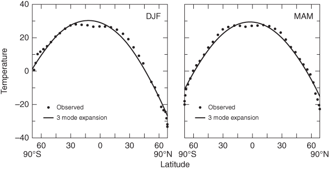
Figure 8.1 Observed zonally averaged surface temperatures of the symmetrized (dots) and the representation of the surface temperatures obtained with the 00, 11, and 20 modes (solid curves). The mode labels are: first digit is the Legendre index, the second digit is the harmonic (0 = mean annual, 1 = annual harmonic).
(North and Coakley (1979). © American Meteorological Society. Used with permission.)
The model consists of two dependent variables ![]() and
and ![]() , the land and ocean surface temperatures averaged around the appropriate segments of their latitude belts. The two energy balance equations are distinguished by the use of
, the land and ocean surface temperatures averaged around the appropriate segments of their latitude belts. The two energy balance equations are distinguished by the use of ![]() and
and ![]() the heat capacities over land and ocean. The governing equation for land is
the heat capacities over land and ocean. The governing equation for land is

where the term ![]() indicates that the heat is transferred from ocean to land proportionally to the difference in those temperatures at the same latitude, but averaged only over the land fraction (hence, the denominator
indicates that the heat is transferred from ocean to land proportionally to the difference in those temperatures at the same latitude, but averaged only over the land fraction (hence, the denominator ![]() ). The ocean equation is similar. The temperature as seen in Figure 8.1 is
). The ocean equation is similar. The temperature as seen in Figure 8.1 is
The three mode amplitudes are governed by the system of equations:

and
By adjusting the value of the land–sea coupling ![]() to 0.226 and the heat capacity over land
to 0.226 and the heat capacity over land ![]() year, one brings the amplitude of
year, one brings the amplitude of ![]() to the observed value of 15.5 K. Since the phase lag is about a week too long, one can further reduce
to the observed value of 15.5 K. Since the phase lag is about a week too long, one can further reduce ![]() to such a value that both the amplitude and phase of
to such a value that both the amplitude and phase of ![]() match the data. The ocean amplitude is only about 3 K for a value of
match the data. The ocean amplitude is only about 3 K for a value of ![]() years and the phase lag is 3 months. Note that for an infinitely deep ocean the phase lag would be a quarter of a cycle and that happens to be 3 months. This says that for our problem of forcing at the 1 year period, this mixed-layer model responds with a phase lag as though the mixed layer were infinitely deep. The seasonal cycle amplitude of the land and/or zonal average temperature is insensitive to the size of
years and the phase lag is 3 months. Note that for an infinitely deep ocean the phase lag would be a quarter of a cycle and that happens to be 3 months. This says that for our problem of forcing at the 1 year period, this mixed-layer model responds with a phase lag as though the mixed layer were infinitely deep. The seasonal cycle amplitude of the land and/or zonal average temperature is insensitive to the size of ![]() .
.
Further experiments with a symmetrized SH show that the same values of these parameters serve to fit the SH seasonal cycle as well. The BBM is interesting, but suffers from too many choices about the phenomenological (adjustable) parameters. Its success in the examples of North and Coakley (1979) are suggestive that a fully two-dimensional model might just work in simulating the seasonal cycle. Before we undertake this task, we must introduce basis functions that will be useful on the two-dimensional plane and then the spherical surface. These steps form the building blocks and generalize from the Legendre polynomials already considered in previous chapters.
8.2 Eigenfunctions in the Bounded Plane
Before tackling the sphere it is useful to solve a simpler eigenvalue problem with less forbidding geometry and with constant heat diffusion coefficient. Imagine our climate to be the temperature distribution on a flat square whose corners are at (0, 0), (0, 1), (1, 1) and (1, 0) in the ![]() plane. The appropriate operator for the heat transport term (divergence of heat flux) in an EBM is
plane. The appropriate operator for the heat transport term (divergence of heat flux) in an EBM is

We seek the eigenfunctions defined by

subject to boundary conditions that we will take to be zero on the boundaries:
where ![]() is an eigenfunction with index
is an eigenfunction with index ![]() and
and ![]() is the corresponding eigenvalue.
is the corresponding eigenvalue.
We proceed by using the method of separation of variables. This consists of making the assumption that the solution for a particular eigenfunction is factorable into a part that is a function only of ![]() and a part that is a function only of
and a part that is a function only of ![]() :
:
Substituting into (8.7) and dividing by ![]() we have
we have

The first term is a function only of ![]() and the second is a function only of
and the second is a function only of ![]() . The only way these functions can be independent of each other and have this dependence is for each to be equal to a constant. First consider the
. The only way these functions can be independent of each other and have this dependence is for each to be equal to a constant. First consider the ![]() -dependent term:
-dependent term:

where we have taken the separation constant to be ![]() , anticipating that it will need to be negative. The solution to this class of ODEs is
, anticipating that it will need to be negative. The solution to this class of ODEs is
where ![]() and
and ![]() are arbitrary constants. To fit the boundary conditions, we must have
are arbitrary constants. To fit the boundary conditions, we must have ![]() . In addition, we must force
. In addition, we must force ![]() to be such that
to be such that ![]() = 0. This can be accomplished by setting
= 0. This can be accomplished by setting ![]() where
where ![]() . We then have
. We then have
where now the index ![]() is used to distinguish the fact that we have a separate function for each (positive) integer value of
is used to distinguish the fact that we have a separate function for each (positive) integer value of ![]() . We can choose the value of
. We can choose the value of ![]() to normalize the functions:
to normalize the functions:

Consider next the ![]() equation:
equation:
where
By applying the same procedure on the boundaries, we find
This implies
where we have replaced the index ![]() by the double index
by the double index ![]() to indicate that actually two integers are involved in specifying the eigenvalue. After normalizing both eigenfunctions, we have
to indicate that actually two integers are involved in specifying the eigenvalue. After normalizing both eigenfunctions, we have
Note that these eigenfunctions individually satisfy the boundary conditions and they are orthonormal.

In addition, the eigenfunctions satisfy a condition known as the completeness relation:

We note that a two-dimensional problem on a finite domain requires two discrete indices for its specification. It is interesting that there is a degeneracy in the eigenvalues, in that two eigenfunctions ![]() and
and ![]() have the same eigenvalue:
have the same eigenvalue: ![]() . This degeneracy is traceable to the invariance of the problem under finite rotation about the domain center by 90
. This degeneracy is traceable to the invariance of the problem under finite rotation about the domain center by 90![]() . Such rotational symmetries always lead to degeneracy of eigenvalues (more than one eigenfunction belonging to the same eigenvalue).
. Such rotational symmetries always lead to degeneracy of eigenvalues (more than one eigenfunction belonging to the same eigenvalue).
The last two equations imply that an arbitrary reasonably well-behaved (it can have simple discontinuities) function ![]() can be expanded into the eigenfunctions:
can be expanded into the eigenfunctions:

Knowing the eigenfunctions allows us to solve many boundary value problems on the same domain having the same boundary conditions. For example, the EBM-like problem
(![]() is a constant with dimension (length)
is a constant with dimension (length)![]() ) on the square with the same boundary conditions as above (the edges are in contact with a reservoir held at 0
) on the square with the same boundary conditions as above (the edges are in contact with a reservoir held at 0 ![]() C) can be solved by expanding
C) can be solved by expanding ![]() and the heat source
and the heat source ![]() into the eigenfunctions, then multiplying through by
into the eigenfunctions, then multiplying through by ![]() and integrating over the square. We are left with an equation for each
and integrating over the square. We are left with an equation for each ![]() and
and ![]() :
:

and finally,

which is the complete solution to the problem. Figure 8.2 shows the first four modal shapes for the square plate.

Figure 8.2 Shapes of the eigenmodes ( ) on a square plate with zero boundary conditions at the edges.
(© Amer. Meteorol. Soc., with permission.)
8.3 Eigenfunctions on the Sphere
8.3.1 Laplacian Operator on the Sphere
The divergence of heat flux for a linear heat conductor with constant thermal conductivity is the Laplacian operator ![]() . In spherical coordinates, this is
. In spherical coordinates, this is

Consider now the eigenfunctions of the two-dimensional Laplacian operator
The functions ![]() will have to be indexed as we shall soon see. As before, each eigenfunction
will have to be indexed as we shall soon see. As before, each eigenfunction ![]() will have an eigenvalue
will have an eigenvalue ![]() that will also have an index label. Our strategy will be to assume that
that will also have an index label. Our strategy will be to assume that ![]() can be factored into
can be factored into
We are again using the method of separation of variables. Inserting this form into the defining equation,
Dividing through by ![]() leads to
leads to

8.3.2 Longitude Functions
Note3 that the left-hand side is a function only of ![]() and the right-hand side is a function only of
and the right-hand side is a function only of ![]() . The only way this can be so is if each side is a constant, which we set arbitrarily equal to
. The only way this can be so is if each side is a constant, which we set arbitrarily equal to ![]() . First consider the right-hand side:
. First consider the right-hand side:

We can now find the solution for ![]()
where ![]() and
and ![]() are arbitrary constants. Note that in order for
are arbitrary constants. Note that in order for ![]() to be single valued,
to be single valued, ![]() must be an integer.
must be an integer.
8.3.3 Latitude Functions
We turn to the longitude-dependent equation that now becomes

It is clear that ![]() needs an index that indicates it is for the particular integer
needs an index that indicates it is for the particular integer ![]() . There is yet to come an index associated with the discretization of
. There is yet to come an index associated with the discretization of ![]() . Anticipating the result, we set
. Anticipating the result, we set ![]() .
.

When appropriately normalized, these ![]() are known as the associated Legendre Functions.
are known as the associated Legendre Functions.
In finding an explicit form for the associated Legendre functions, the first step is to substitute
After substituting, we arrive finally at the differential equation for ![]() :
:
We proceed as in the last chapter with the assumption that ![]() can be written as a power series:
can be written as a power series:

Similar to what we did earlier, after some manipulation, we arrive at the recursion formula for the coefficients ![]() :
:

Hence, if ![]() and
and ![]() are provided, the rest of the coefficients are determined. As before, we encounter the divergence problem unless the numerator above cuts off at some level so that the rest of the terms vanish and
are provided, the rest of the coefficients are determined. As before, we encounter the divergence problem unless the numerator above cuts off at some level so that the rest of the terms vanish and ![]() becomes a finite-degree polynomial. We find that this will happen if
becomes a finite-degree polynomial. We find that this will happen if ![]() . In other words,
. In other words, ![]() must be an integer larger than or equal to
must be an integer larger than or equal to ![]() . We break up the functions into odd- or even-order polynomials, depending upon whether
. We break up the functions into odd- or even-order polynomials, depending upon whether ![]() is odd or even. When it is even, we choose
is odd or even. When it is even, we choose ![]() and proceed to have an even polynomial. When
and proceed to have an even polynomial. When ![]() is odd, we set
is odd, we set ![]() and proceed to have an odd-order polynomial. We now have a prescription for finding the
and proceed to have an odd-order polynomial. We now have a prescription for finding the ![]() . Hence, we may write
. Hence, we may write
![]()
By convention, we simplify the notation further by letting ![]() run from
run from ![]() to
to ![]() , then we can also define the
, then we can also define the ![]() , and we must then restrict
, and we must then restrict ![]() . This allows us to write
. This allows us to write
Note that the normalization ![]() can be chosen such that
can be chosen such that
It is possible to show by direct substitution into the defining differential equation the important rule

If we employ Rodrigues' formula for the ![]() ,
,

we can show

which leads to evaluation of the aforementioned proportionality coefficient:

It is possible to derive an orthogonality relation for the ![]() when the
when the ![]() values agree:
values agree:

8.4 Spherical Harmonics
We define the functions4

where we have used the shorthand notation ![]() to stand for the point on the sphere corresponding to
to stand for the point on the sphere corresponding to ![]() . From this definition, we can establish
. From this definition, we can establish
8.4.1 Orthogonality
Normalization and orthogonality conditions are then

where we have used the further shorthand notation ![]() , the element of solid angle on the Earth's surface. Another important relation is the completeness relation:
, the element of solid angle on the Earth's surface. Another important relation is the completeness relation:

The first few spherical harmonics are


Figure 8.3 shows contour maps of the real and imaginary parts of ![]() .
.

Figure 8.3 Shapes of the real and imaginary parts of the first few spherical harmonics. (a) Re( ; (b) Im(
 ); (c) Re(
 ; (d) Im(
 ); (e) Re
 ); (f) Im(
 ).
).
8.4.2 Truncation
The truncation level of an eigenfunction expansion usually can be associated with a level of smoothing. In the case of a spherical harmonic expansion on the sphere, we have two indices ![]() and
and ![]() representing longitudinal and latitudinal levels in the series. There are good reasons to truncate the series at some value of
representing longitudinal and latitudinal levels in the series. There are good reasons to truncate the series at some value of ![]() , the degree of the spherical harmonic at the end of the series. This is known as triangular truncation. It is indicated schematically in Figure 8.4a. Also shown in Figure 8.4b is a truncation known as rhomboidal truncation. This latter truncation was used in some early numerical models of the atmosphere. Nearly all spherical harmonic representations are truncated in the triangular form today.
, the degree of the spherical harmonic at the end of the series. This is known as triangular truncation. It is indicated schematically in Figure 8.4a. Also shown in Figure 8.4b is a truncation known as rhomboidal truncation. This latter truncation was used in some early numerical models of the atmosphere. Nearly all spherical harmonic representations are truncated in the triangular form today.
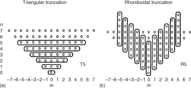
Figure 8.4 Truncating a spherical harmonic expansion. Each panel shows an array of 0s with the vertical column labeled by the degree  and the horizontal representing the longitudinal index
  . Each 0 in the diagram represents a term retained in the truncated series. (a) Illustration of how the triangular truncation works in an example labeled T5. (b) alternative rhomboidal truncation, denoted by R5.
Figure 8.5 gives a further idea of the way spatial scales are included in a T3 truncation. Note in the figure the different phasing between the imaginary part in the top row of components. The vertical column entries at ![]() are just the Legendre polynomials.
are just the Legendre polynomials.
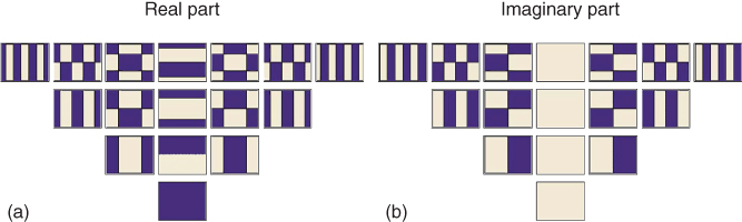
Figure 8.5 Triangular (T3) diagram showing the real part of spherical harmonic patterns in (a) and the imaginary part in (b) up to T3. The dark shading indicates positive values.
8.5 Solution of the EBM with Constant Coefficients
We are now in a position to solve the energy balance equation on the sphere when the coefficients are not functions of position. We consider the spherical harmonic series expansion

The energy balance equation reads
where now we have allowed for the possibility of ![]() and
and ![]() to depend on
to depend on ![]() and
and ![]() . Inserting the Laplace series expansion, we have
. Inserting the Laplace series expansion, we have

where

The special case for which the time dependence of ![]() and
and ![]() is suppressed leads to the equilibrium solution,
is suppressed leads to the equilibrium solution,

If we perturb the solution from equilibrium, we find the interesting result for uncoupled exponential decay modes with time constants given by
In other words, the decay time for mode ![]() depends only on the degree
depends only on the degree ![]() and not on the longitudinal wave number
and not on the longitudinal wave number ![]() .
.
8.6 Introducing Geography
In this section, we briefly introduce the geographical input that we will use extensively later. Consider the possibility that the heat capacity density ![]() depends upon position on the globe,
depends upon position on the globe, ![]() . It is reasonable that
. It is reasonable that ![]() depends strongly on whether the surface type is continental or oceanic. For an all-land planet we have seen that in many applications, the time constant can be taken to be about 30 days, as that is roughly equivalent to taking about half of the Earth's atmospheric mass into account. On the other hand, over ocean, heat mixes very quickly (few days) down to a depth of about 80 m. This means that the amount of mass involved is about 60 times as much as in the atmosphere alone. One way to account for geography in these models is to let
depends strongly on whether the surface type is continental or oceanic. For an all-land planet we have seen that in many applications, the time constant can be taken to be about 30 days, as that is roughly equivalent to taking about half of the Earth's atmospheric mass into account. On the other hand, over ocean, heat mixes very quickly (few days) down to a depth of about 80 m. This means that the amount of mass involved is about 60 times as much as in the atmosphere alone. One way to account for geography in these models is to let ![]() take on these drastically different magnitudes depending upon the local surface type. Let us take
take on these drastically different magnitudes depending upon the local surface type. Let us take ![]() days over land surfaces and
days over land surfaces and ![]() years over oceanic surfaces. This leads to a strongly position-dependent step function at the continental borders all around the spherical surface. A handy way to incorporate this in our formulation is to expand in a Laplace series
years over oceanic surfaces. This leads to a strongly position-dependent step function at the continental borders all around the spherical surface. A handy way to incorporate this in our formulation is to expand in a Laplace series

where ![]() is the triangular truncation degree. By not carrying the sum to
is the triangular truncation degree. By not carrying the sum to ![]() and truncating it at a finite level, we have effectively smoothed out some of the sharp edges in the function – the truncation acts like a smoothing filter, excluding features smaller than a certain size inversely proportional to
and truncating it at a finite level, we have effectively smoothed out some of the sharp edges in the function – the truncation acts like a smoothing filter, excluding features smaller than a certain size inversely proportional to ![]() (recall that
(recall that ![]() is the number of zeros from pole to pole in
is the number of zeros from pole to pole in ![]() ). Figure 8.6 shows contour maps of
). Figure 8.6 shows contour maps of ![]() at two different degrees of truncation. There is some arbitrariness in the way one truncates a Laplace series. In atmospheric science, there have appeared two truncation conventions: the rhomboidal and the triangular. The triangular is easiest as it is the one we have used in the previous sections.
at two different degrees of truncation. There is some arbitrariness in the way one truncates a Laplace series. In atmospheric science, there have appeared two truncation conventions: the rhomboidal and the triangular. The triangular is easiest as it is the one we have used in the previous sections.

is known as triangular truncation at degree ![]() or simply
or simply ![]() . Most atmosphere/ocean climate model simulations cited in the recent Intergovernmental Panel on Climate Change (IPCC) reports require at least a resolution of T84. Typical weather forecast models at the time of this writing are at T200+. The advantage of triangular truncation is that this truncation preserves some of the rotational symmetry properties associated with the spherical harmonics. For example, under a rotation of the spherical coordinate system, the members of a given
. Most atmosphere/ocean climate model simulations cited in the recent Intergovernmental Panel on Climate Change (IPCC) reports require at least a resolution of T84. Typical weather forecast models at the time of this writing are at T200+. The advantage of triangular truncation is that this truncation preserves some of the rotational symmetry properties associated with the spherical harmonics. For example, under a rotation of the spherical coordinate system, the members of a given ![]() multiplet transform into each other. This is a useful property as will be seen in a later chapter on fluctuations on the uniform sphere.
multiplet transform into each other. This is a useful property as will be seen in a later chapter on fluctuations on the uniform sphere.
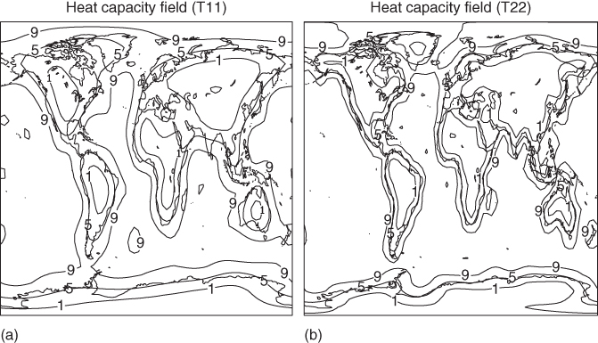
Figure 8.6 Contour map of  truncated at (a) spherical harmonic degree 11 and (b) degree 22.
An alternative way of truncating the series that has been utilized in many early general circulation models is the rhomboidal truncation. In this case, we reverse the order of the summation:

We call this rhomboidal truncation at level ![]() or simply
or simply ![]() . The two methods of summation are compared in the diagram in Figure 8.4. The advantage of rhomboidal truncation has been mostly computational. The length of the columns in the figure are clearly equal in this scheme and this has been useful in efficiently vectorizing some computer algorithms in the numerical solutions.
. The two methods of summation are compared in the diagram in Figure 8.4. The advantage of rhomboidal truncation has been mostly computational. The length of the columns in the figure are clearly equal in this scheme and this has been useful in efficiently vectorizing some computer algorithms in the numerical solutions.
8.7 Global Sinusoidal Forcing
Consider the two-dimensional EBM forced by a sinusoidal forcing function in time by modifying the outgoing radiation constant term:
This is similar to a global forcing by such an agent as greenhouse gas forcing, but we will allow it to be sinusoidal in time. Similarly to an engineer probing a black box, we drive the electrodes of the box with a sinusoidal forcing and study the response amplitude and phase lag. We can insert this forcing into our governing equation and as the temperature responds at the same frequency as the forcing,
with ![]() a complex function of position only. After canceling the common exponential factor, we have
a complex function of position only. After canceling the common exponential factor, we have
This means that each frequency component of the temperature field is uncoupled from every other one. On the other hand, we now find that because of the presence of the spatial dependence of ![]() , the situation is much more complicated than in the rotationally invariant cases studied in previous sections. Inserting the Laplace series for
, the situation is much more complicated than in the rotationally invariant cases studied in previous sections. Inserting the Laplace series for ![]() and
and ![]() , we obtain
, we obtain

Now, on multiplying through by ![]() and integrating over the sphere, we encounter some new objects:
and integrating over the sphere, we encounter some new objects:

the so-called spherical harmonic coupling coefficients. The result is

where the coupling matrix ![]() is given by
is given by
In principle, the matrix ![]() has an inverse so that, formally,
has an inverse so that, formally,

or, in more compact form,

This is the formal solution to the problem. The matrix ![]() has to be computed by first obtaining
has to be computed by first obtaining ![]() from a map of the land–sea geography, then it must be expanded into the
from a map of the land–sea geography, then it must be expanded into the ![]() and finally this must be combined with values of the
and finally this must be combined with values of the ![]() (from readily available tables or computer algorithms). The matrix
(from readily available tables or computer algorithms). The matrix ![]() also depends on the driving frequency
also depends on the driving frequency ![]() . Since the complex element
. Since the complex element ![]() appears explicitly, the matrix
appears explicitly, the matrix ![]() is a complex matrix that has to be inverted on a computer. Once the geography is set, the list
is a complex matrix that has to be inverted on a computer. Once the geography is set, the list ![]() are fixed once and for all. The
are fixed once and for all. The ![]() are only computed once and stored. However, the linear weighting of these in the computation of
are only computed once and stored. However, the linear weighting of these in the computation of ![]() will depend on forcing frequency
will depend on forcing frequency ![]() , requiring that
, requiring that ![]() be reinverted for each experiment
be reinverted for each experiment ![]() .
.
Once the complex amplitude ![]() has been computed, we must recompose the Laplace series to obtain the complex function
has been computed, we must recompose the Laplace series to obtain the complex function ![]() . The magnitude or modulus of this function tells us the amplitude of the response at the point
. The magnitude or modulus of this function tells us the amplitude of the response at the point ![]() on the Earth. The phase of the complex function at
on the Earth. The phase of the complex function at ![]() tells us the phase lag in radians behind the forcing phase.
tells us the phase lag in radians behind the forcing phase.
It is instructive to examine the behavior of the amplitude of the response as a function of position on the Earth at different forcing frequencies. Figure 8.7 shows response amplitude maps for four different frequencies (indicated by their periods). The amplitude of the forcing was chosen such that it corresponds roughly to a doubling of ![]() (
(![]() W m
W m![]() ). The equilibrium response (
). The equilibrium response (![]() ) to this forcing should be about
) to this forcing should be about ![]() . Figure 8.7a indicates that the amplitude is large over the large continental interiors because the thermal inertia (
. Figure 8.7a indicates that the amplitude is large over the large continental interiors because the thermal inertia (![]() ) is smaller in those locations. As the period of the forcing is increased (Figure 8.7b–d), the amplitude of the response becomes more uniform over the globe. The relevant parameter is the relaxation time of the particular surface compared to the period of the forcing. Observe that the length scale in the response field increases with longer periods of forcing.
) is smaller in those locations. As the period of the forcing is increased (Figure 8.7b–d), the amplitude of the response becomes more uniform over the globe. The relevant parameter is the relaxation time of the particular surface compared to the period of the forcing. Observe that the length scale in the response field increases with longer periods of forcing.

Figure 8.7 Illustration of the response to sinusoidal forcing by  at different periods. Shown are the contour maps of amplitude of response for a sinusoidal
  doubling. All four cases are shown for easy comparison: (a) Period = 2 months; (b) Period = 1 year; (c) Period = 8 years; (d) Period = 24 years. As the period of the forcing increases, the spatial pattern of the response increases in scale.
8.8 Two-Dimensional Linear Seasonal Model
The two-dimensional model can be formulated as in the previous chapter, only here we allow for the spatial dependence of thermal diffusion, ![]() . We make Laplace–Fourier expansions of the quantities
. We make Laplace–Fourier expansions of the quantities
for insertion into the EBM
This model has been solved (North et al., 1983; Hyde et al., 1989) and the solutions recovered by the very same technique as in the last chapter except that the model must be solved separately for each temporal harmonic ![]() . Once the mode amplitudes
. Once the mode amplitudes ![]() ,
, ![]() have been found by inverting the response matrix for each
have been found by inverting the response matrix for each ![]() , the solution field can be recomposed from the aforementioned.
, the solution field can be recomposed from the aforementioned.
8.8.1 Adjustment of Free Parameters
The model now has several new parameters whose values must be determined by fitting to the present seasonal cycle. The diffusion parameter has the form (Mengel et al., 1988)
Different values of the parameters ![]() , and
, and ![]() have been used in different publications over the years. The function
have been used in different publications over the years. The function ![]() is plotted in Figure 8.8 with the solid line representing the thermal conductivity used by Mengel et al. (1988) and Kim and North (1992) and the short dashed curve is form used by Graves et al. (1993). The long-dashed line is the constant value used in Chapter 5 in fitting the one dimensional model. The coefficients
is plotted in Figure 8.8 with the solid line representing the thermal conductivity used by Mengel et al. (1988) and Kim and North (1992) and the short dashed curve is form used by Graves et al. (1993). The long-dashed line is the constant value used in Chapter 5 in fitting the one dimensional model. The coefficients ![]() , and
, and ![]() had to be adjusted to give a reasonable fit to the present seasonal cycle. One conjecture is that the diffusion parameter has to be larger in the tropics to account for the larger vapor pressure of water there and the increased efficiency of the Hadley cell (Lindzen and Farrell, 1977).
had to be adjusted to give a reasonable fit to the present seasonal cycle. One conjecture is that the diffusion parameter has to be larger in the tropics to account for the larger vapor pressure of water there and the increased efficiency of the Hadley cell (Lindzen and Farrell, 1977).
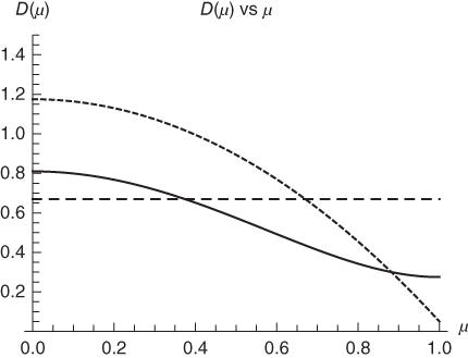
Figure 8.8 Illustration of the choices of the latitude dependence of diffusion coefficient in different models, with the diffusion parameter  as a function of
  . The long-dashed curve is the choice used in the one-dimensional model of Chapter 5, the solid curve is from Mengel et al. (1988) and Kim and North (1992), and the short-dashed curve is from Graves et al. (1993), who took
  , by adjusting
  to a smaller value. An alternative not considered was to give
  a latitude dependence and keeping
  a constant.
Another problem with the simulations is that the Arctic Ocean is mostly covered with sea ice. This has the heat capacity of neither land nor sea. Hence, we must introduce another step in the step function ![]() to account for the fact that sea ice has puddles, open cracks (leads), and other features that are not easily modeled in the linear form we have taken. Nevertheless, we attempt to take these into account in the present context by simply assigning those areas with perennial sea ice to have a value of
to account for the fact that sea ice has puddles, open cracks (leads), and other features that are not easily modeled in the linear form we have taken. Nevertheless, we attempt to take these into account in the present context by simply assigning those areas with perennial sea ice to have a value of ![]() . This last value came from adjusting its magnitude until the annual harmonic of the surface temperature field came into agreement with the data.
. This last value came from adjusting its magnitude until the annual harmonic of the surface temperature field came into agreement with the data.
8.9 Present Seasonal Cycle Comparison
The next three subsections contain discussions on how the model simulates the annual and semiannual harmonics of the surface temperature field. In these simulations, the seasonal cycle forcing includes the important semiannual harmonic contribution to the second Legendre polynomial mode ![]() . This term makes an important contribution especially near the equator over which the Sun passes twice a year. It also contributes significantly in the polar regions where there is perpetual darkness in winter and perpetual daylight in summer. The convergence of the Fourier–Laplace series is slow in the polar regions because of the discontinuous derivative at the latitude of perpetual day (or night). Including this additional term improves the behavior in those regions.
. This term makes an important contribution especially near the equator over which the Sun passes twice a year. It also contributes significantly in the polar regions where there is perpetual darkness in winter and perpetual daylight in summer. The convergence of the Fourier–Laplace series is slow in the polar regions because of the discontinuous derivative at the latitude of perpetual day (or night). Including this additional term improves the behavior in those regions.
8.9.1 Annual Cycle
The amplitude of the annual cycle agrees well with the smoothed data as seen in Figure 8.9. The agreement is especially noteworthy over the two Northern Hemisphere continents. It is interesting that the data indicate a hint of the Himalayan plateau but the model has no such feature because no allowance is made in this model for topography. The agreement is also good in and around Antarctica. The tiny 1 K amplitude curves in the tropics show some conformity with the observations. The overall coincidence of the contours with the continental boundaries is indicative of the very strong influence of the land–sea contrast in heat capacity. The phase lag is more sensitive to local geography and it is not mimicked as well as seen in Figure 8.10. First, the phase lag in the tropics should be ignored as the annual harmonic is very small in the model and in the data. The phase lag of about or less than 30 days in the interior of each Northern Hemisphere continent is very good except for some details. In North America, the 30 days contour is obviously influenced by the Rocky Mountain chain. There is similar disagreement that is easily explained over the mountains in South America (both due to shorter lags over high terrain). A similar high plateau erroroccurs over the Himalayas. Agreement over the ocean is moderate, being more extreme in the model regarding the quarter cycle (90 days) lag. We conclude that the annual cycle is modeled rather well except for some features that are not expected to be faithfully represented in such a comparison.

Figure 8.9 Plots illustrating the agreement of the modeled versus observed first harmonic of the seasonal cycle. Shown are contour plots of the amplitude of the surface temperature field of the annual harmonic. (a) From observations as determined from smoothed data by truncating the spherical harmonic expansion at T11. (b) The same as in (a) except for the two-dimensional EBCM. Contours are in intervals of 5 K except for the 1 K curve.
(Kim and North (1992). Reproduced with permission of Wiley.)

Figure 8.10 Plots featuring the agreement of the modeled versus observed first harmonic phase lag of the seasonal cycle. Shown are contour plots of the phase lag (days) of the annual harmonic. (a) From observations as determined from smoothed data by truncating the spherical harmonic expansion at T11. (b) The same as (a) except for the two-dimensional EBCM. Note that over large land masses, the phase lag is about 1 month while over large ocean expanses the lag is 2–3 months.
(Kim and North (1992). Reproduced with permission of Wiley.)
8.9.2 Semiannual Cycle
The first thing to notice about the semiannual cycle as shown in Figure 8.11 is how small it is. This is indicative of the rapid convergence of the Fourier series representing the seasonal surface temperature field. Over ocean surfaces, it is smaller than 1 K except in polar regions, where, as noted above, it feels the second harmonic forcing from the polar day/night term. This same day/night forcing of the amplitude over polar regions, especially Antarctica, leads to large responses over both model and data.

Figure 8.11 Contour plot of the surface temperature field of the semiannual harmonic. (a) From observations as determined from smoothed data by truncating the spherical harmonic expansion at T11. (b) The same as (a) except for the two-dimensional EBCM. The semiannual harmonic is important in the tropics and in the polar regions. In the polar regions, this is the first correction toward resolving the polar day and night features. This graphic also helps to indicate the rapid convergence of the Fourier series in time.
(Kim and North (1992). Reproduced with permission of Wiley.)
8.10 Chapter Summary
The expansion of EBCMs from one to two dimensions on the spherical surface was first motivated by a discussion of the BBM, which is a planet with continents whose borders are pole to pole along meridians. This led to a model that is symmetric across the equator. An EBCM was concocted that mimicked a symmetrized NH. The effective heat capacities of land and sea along with a parameter that coupled ocean and land temperatures at the same latitudes could be adjusted to form a seasonal cycle of the model that agreed with the seasonal cycle of observations. The fact that the data could be well represented by three Legendre polynomial modes (![]() ), where the seasonal cycle is carried only by mode index unity, and that mode was sinusoidal in time suggested that this simple approach was on the right track. Unfortunately, the BBM required too many adjustable parameters for it to be useful.
), where the seasonal cycle is carried only by mode index unity, and that mode was sinusoidal in time suggested that this simple approach was on the right track. Unfortunately, the BBM required too many adjustable parameters for it to be useful.
The next step was clearly to try allowing the heat capacity to be a function of position on the sphere: ![]() . Before building the model, we introduced two-dimensional eigenfunctions of the Laplace operator (
. Before building the model, we introduced two-dimensional eigenfunctions of the Laplace operator (![]() ), first on a plane square then onto the sphere, where we encounter the spherical harmonics. Spherical harmonics turn out to be the modal shapes of the EBCM if the heat capacity function
), first on a plane square then onto the sphere, where we encounter the spherical harmonics. Spherical harmonics turn out to be the modal shapes of the EBCM if the heat capacity function ![]() is not a function of position. When it is a function of position, we must resort to numerical methods. This has been carried out by many studies over the last three decades by a number of different numerical approaches (North et al., 1983; Hyde et al., 1989; Bowman and Huang, 1991; Kim and North, 1991; Stevens and North, 1996; North and Wu, 2001; Zhuang et al., 2014).
is not a function of position. When it is a function of position, we must resort to numerical methods. This has been carried out by many studies over the last three decades by a number of different numerical approaches (North et al., 1983; Hyde et al., 1989; Bowman and Huang, 1991; Kim and North, 1991; Stevens and North, 1996; North and Wu, 2001; Zhuang et al., 2014).
The solutions to the two-dimensional model, as shown, were obtained by analyzing the model and data into mean annual, annual harmonic, and semi-nnual harmonic as a function of position. The Fourier series of these harmonics converges very rapidly so that only these few harmonics are necessary to obtain a very good representation of both model and data. The shape of the annual cycle fits the data extremely well with large amplitude over land masses and smaller ones over the ocean surfaces. The phase lag between insulation and response of the annual harmonic is only about 1 month over the interiors of the large continents and roughly three months over the ocean surfaces. While some details differ, the gross features of the phase lag are captured. The semiannual harmonic amplitude is also in very good agreement with the data with very small amplitude (![]() K) over most of the globe but larger as one approaches either pole.
K) over most of the globe but larger as one approaches either pole.
The general success of the two-dimensional EBCM suggests that it might be good enough for some applications in paleoclimatology and others such as designing observational networks or in detection of climate signals. Given the success of the two-dimensional EBCM in simulating the seasonal cycle,we push the two-dimensional EBCM to include random (weather noise) forcing.
Notes for Further Reading
The book by Washington and Parkinson (2005) discusses spherical harmonics in the context of three-dimensional climate models, as well as numerical methods for general circulation models. Most books on mathematical physics such as Arfken and Weber (2005) discuss linear boundary value problems and the use of spherical harmonics and other special functions.
Exercises
- 8.1
- a. Show that the eigenvalue problem

- allows a solution in the form

- Determine the corresponding eigenvalue.
- b. Determine the solution of

- with boundary conditions

- a. Show that the eigenvalue problem
- 8.2 Show that the solution of

with boundary conditions

is given by

where

- 8.3 Prove by deduction that

- 8.4 The Poisson equation in spherical coordinates is give by

where
 is longitude and
  is latitude. Boundary conditions are given by
Obtain a zonally symmetric solution of the Poisson equation.
- 8.5 Consider the Laplace equation in spherical coordinates:

where
 is longitude,
  is co-latitude, and
  is radius.
- a. Assuming a separable solution,
 , rewrite the Laplace equation above in terms of the separable solution.
 - b. Let us assume a radial solution in the form
 , rewrite the governing equation in Part (a).
 - c. Set up the equation for a zonally symmetric solution. Solve the resulting problem.
- d. Without the assumption of zonal symmetry, a separable solution of the equation in Part (b) can be written as
 . Use the result in Part (c), set up the governing equation for each component of the separable solution. Obtain the longitudinal component of the solution.
 - e. Let us assert that the solution for the latitudinal component of the equation is given by

- where
 is called the associated Legendre function of order
  and rank
  . Prove that the associated Legendre function satisfies latitudinal component of the Laplace equation.
- a. Assuming a separable solution,
- 8.6 Legendre functions are generated by using

which is known as the Rodrigues' formula. Using the formula, generate the Legendre polynomials up to order 4 (
 ).
). - 8.7 For this problem, use the Rodrigues' formula in Exercise 8.6 and the definition of associated Legendre functions in Exercise 8.5.
- a. Develop the Rodrigues' formula for associated Legendre functions.
- b. Show that the associated Legendre functions with a negative rank defined by

- satisfies

- c. Using the Rodrigues' formula in Parts (a) and (b), derive the associated Legendre functions for up to order
 .
.
- 8.8 Spherical harmonic basis functions are the solutions of Laplace equations in spherical coordinates. As discussed in Exercises 8.4 and 8.5, a most general solution is given by

where

is called the spherical harmonics of order
 and rank
  . Any horizontal spatial patterns (at the same elevation
  ) can be decomposed in terms of spherical harmonic basis functions.
- a. Show that

- b. Consider an equilibrium solution of a two-dimensional EBM for a perpetual January 1 simulation with a constant albedo:

- where
 is a unit vector pointing from the center of the planet to a point
  on the surface, the insolation distribution function
  is at its perpetual configuration and
  , and
, and  are simply constants. Set up an EBM equation by using spherical harmonics and obtain a closed-form solution.
- a. Show that