Chapter 12
Applications of EBMs: Paleoclimate
12.1 Paleoclimatology
There are a few areas in paleoclimatology that are particularly well suited for energy balance modeling. It is important to remember that EBMs as we present them in this book (except for those considering vertical structures in Chapters 3 and 4) only treat the surface temperature field. Precipitation and changing ocean circulations are also not included in these EBMs although they are clearly of interest in paleoclimatology. Fortunately, much of the data coming from empirical studies in paleoclimatology pertain to the surface temperature. Anything above the surface is out of bounds for us—it requires a much more sophisticated model to go above the surface or to deal with any transport phenomena such as the transport of water vapor above the boundary layer.
Before plunging into EBM applications directly, we present a very short summary of the Earth's climate history. One of the first problems we encounter is based on sound theoretical evidence of the lower brightness of the Sun at the time of the formation of the Earth and through its settlement into a planet with land and ocean surfaces. According to long-accepted astrophysical theory, the Sun was only about 70% as bright as it is today. Recalling our study of ice-cap models in Chapters 2 and 7, we see that the evolution of the Earth's climate was quite different from what these models based on a monotonically increasing solar brightness and no changes in atmospheric greenhouse gas might suggest. Bender (2013) and Feulner (2012) review the many theories of how we might avoid the “faint Sun paradox,” according to which the planet could not possibly get to our present climate by a steadily increasing external forcing. The solution must lie in the atmosphere's changing composition—perhaps much more powerful greenhouse gas concentrations came to the rescue—but it would take substantial amount of forcing, perhaps tens of percent of the equivalent of solar brightness.
Ward and Kirschvink (2015) argue that there were incidences of “snowball Earths” as early as 2.2 Ga1 (the so-called Huronian event). They also argue that these events might have been instrumental in the beginnings of life on the planet. This first massive glaciation might have lasted several hundred My. The event was coincident with a large increase (several bars, one bar of pressure = that of one atmosphere) in ![]() in the atmosphere due to oxygenic photosynthesis. There might have been lots of methane in the atmosphere at that time and itmight explain the hot planet preceding the ice event. The oxygenation of the methane might have cooled the planet sufficiently to cause the collapse to the snowball. Other possibilities include the increase of weathering (removal of
in the atmosphere due to oxygenic photosynthesis. There might have been lots of methane in the atmosphere at that time and itmight explain the hot planet preceding the ice event. The oxygenation of the methane might have cooled the planet sufficiently to cause the collapse to the snowball. Other possibilities include the increase of weathering (removal of ![]() ) following accretion of large objects and collisional tectonics (Melezhik, 2006).
) following accretion of large objects and collisional tectonics (Melezhik, 2006).
There is evidence suggesting that there was another interval when the planet was totally ice covered several times, later called the Neoproterozoic period (1 Ga to 542 Ma). These are also periods thought to include total ice cover (Kirschivink, 1992; Evans, 2000; Hoffman and Schrag, 2002) . There is a large literature on this subject; several of these papers tend to confirm the geological dating and resolve issues of global synchronicity for the ice cover. Among these are papers that present pretty sound evidence of tropical glaciers. Our elementary models suggest that, without wild changes in obliquity, it would be hard to have the tropics covered with ice without the whole globe so covered. These glaciations might have persisted for tens of My. The Neoproterozoic glaciations took place after the emergence of life on the planet and one wonders how organisms might have survived. Warren et al. (2002) propose that thin ice cover over the oceans might have allowed the passage of enough sunlight to support photosynthesis. Other papers have been concerned with the survival of multicellular organisms during such inhospitable conditions.
In the Paleozoic era (![]() to 200 Ma), there is evidence of numerous large-scale glaciations (but not snowballs). The continents were going through rearrangements over this and later periods on time scales of millions of years and these configurations of land/sea geography are likely to have played a role in the early ice ages. Figure 12.1 summarizes the geological time intervals to be used in the discussion.
to 200 Ma), there is evidence of numerous large-scale glaciations (but not snowballs). The continents were going through rearrangements over this and later periods on time scales of millions of years and these configurations of land/sea geography are likely to have played a role in the early ice ages. Figure 12.1 summarizes the geological time intervals to be used in the discussion.

Figure 12.1 Geological timescale indicating boundaries separating eons, eras, periods, and epochs along with the times in Ma. Note that the durations of the intervals are not drawn to temporal scale in this chart.
(Data from Bender (2013).)
At around 50 Ma the Earth began to gradually cool (geologically speaking) as shown in Figure 12.2. This figure, modified from the original found in Zachos et al. (2001), and a similar modification featured in Chapter 6 of Bender (2013) tell much about the climate over the last 65 Ma. Bender (2013) describes how the ![]() O record from bottom-dwelling microbiota can be used to infer global temperatures. On the basis of Figure 12.2, we can trace a gradual descent from a much warmer (
O record from bottom-dwelling microbiota can be used to infer global temperatures. On the basis of Figure 12.2, we can trace a gradual descent from a much warmer (![]() C warmer at around 50 Ma, called the early Eocene thermal maximum) planetary surface to that at present. The main governing factor was likely to be
C warmer at around 50 Ma, called the early Eocene thermal maximum) planetary surface to that at present. The main governing factor was likely to be ![]() decreases over this time. As time proceeds, the planet continues to gradually cool until the beginning of the Oligocene epoch (
decreases over this time. As time proceeds, the planet continues to gradually cool until the beginning of the Oligocene epoch (![]() 34 Ma). At this point in time, there is a sharper rate of cooling which is attributed to the growth of continent-wide ice in Antarctica. From that point to the present, the planet has a large (south) polar ice sheet, with Greenland ice coverage likely occurring at the beginning of the Pliocene. The last million years or so (the Pleistocene) features large excursions in ice sheets, most of which occur in the Northern Hemisphere.
34 Ma). At this point in time, there is a sharper rate of cooling which is attributed to the growth of continent-wide ice in Antarctica. From that point to the present, the planet has a large (south) polar ice sheet, with Greenland ice coverage likely occurring at the beginning of the Pliocene. The last million years or so (the Pleistocene) features large excursions in ice sheets, most of which occur in the Northern Hemisphere.
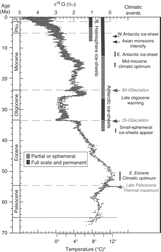
Figure 12.2 Estimates of global temperature (horizontal axis) versus time (vertical axis). The temperature is estimated from  O data collected from benthic foraminifera.
(Zachos et al. (2001). Reproduced with permission of AAAS.)
12.1.1 Interesting Problems for EBMs
- The first problem for EBMs has already come up in Chapter 2 in which we found a possible ice-covered Earth solution to our global energy balance equation. The operating curve showed that if the solar brightness was dropped by only a small percentage, the planet would plunge into a deep-freeze state. Of course, the percentage depends on the details of model parameter choices.
- The second problem is the effect of the land–sea distribution over deep geological time scales where, through continental drift, the landmasses have continuously changed their configurations. It could be that summertime's warmest temperatures determine whether snow will linger over the warm season and allow the growth of an ice field and eventually a large-scale ice sheet. We know that the proximity to the poles and the shapes of landmasses can alter the summertime temperatures. Could EBMs tell us when ice sheets should have been present? The seasonal cycle is a key factor.
- The third concerns the most recent few tens of millions of years during which the Earth has shifted from a warmer state to one with large continental ice sheets, the most prominent being Antarctica and Greenland. What were the conditions for these and what might EBMs have to contribute?
- A fourth has to include the ice sheets that have waxed and waned over North America and Western Europe (but not over Siberia). Observations provide evidence suggesting that the glaciations exhibit a regularity and are in step with the theoretically calculated oscillations of orbital elements of our planet. Might EBMs be of use in understanding the glaciations over the Pleistocene (last few million years), and even the most recent 10 ka, (some authors use 12 ka) called the Holocene?
Not all problems are approachable, not to mention solvable, by EBMs. Atmospheric chemistry and ocean circulation play roles possibly as important as the changing land–sea configuration and the associated radiative-energy-balance effects on summertime temperatures. Sometimes, chemistry and aerosol effects can be inserted into an EBM, but even then the problem might not be solved or may not be interesting. For instance, if atmospheric ![]() increased because of some geological process, the EBM contribution may be large, but it is not the importantaspect of the problem (e.g., why did
increased because of some geological process, the EBM contribution may be large, but it is not the importantaspect of the problem (e.g., why did ![]() increase?). But if the greenhouse gas and aerosol concentrations are given, it is straightforward to provide EBM solutions. Long-lived ocean current anomalies or surface temperature aberrations (e.g., a shift in the Gulf Stream) can be included by prescribing them, but as yet no one has found a way to include them dynamically in such a simple model. Unfortunately for the EBM aficionado, the use of a general circulation model (GCM) may be far more appropriate for such a forcing as they are likely to excite interesting quasi-stationary wave patterns that affect storm paths (all this is outside the scope of an EBM). As we found in Chapter 10, we can include some oceanic effects in EBMs, but to attempt the circulation of the ocean currents is well beyond the scope of simulation at this level of the model hierarchy. Perhaps the single, most important advantage for EBMs is to spell out how the seasonal cycle can play a role in various paleoclimate problems, as the seasonal cycle responds almost linearly to forcings due to changes in orbital elements,
increase?). But if the greenhouse gas and aerosol concentrations are given, it is straightforward to provide EBM solutions. Long-lived ocean current anomalies or surface temperature aberrations (e.g., a shift in the Gulf Stream) can be included by prescribing them, but as yet no one has found a way to include them dynamically in such a simple model. Unfortunately for the EBM aficionado, the use of a general circulation model (GCM) may be far more appropriate for such a forcing as they are likely to excite interesting quasi-stationary wave patterns that affect storm paths (all this is outside the scope of an EBM). As we found in Chapter 10, we can include some oceanic effects in EBMs, but to attempt the circulation of the ocean currents is well beyond the scope of simulation at this level of the model hierarchy. Perhaps the single, most important advantage for EBMs is to spell out how the seasonal cycle can play a role in various paleoclimate problems, as the seasonal cycle responds almost linearly to forcings due to changes in orbital elements, ![]() , and aerosol concentrations, as well as the geographical distribution of land and sea. These concepts have been a common theme in the many works of Crowley and his colleagues Hyde, Baum, and Short (for a list of others see the preface of this book.).
, and aerosol concentrations, as well as the geographical distribution of land and sea. These concepts have been a common theme in the many works of Crowley and his colleagues Hyde, Baum, and Short (for a list of others see the preface of this book.).
12.2 Precambrian Earth
The Earth settled into its present form with an atmosphere including distinctly defined ocean and landmasses a few billions of years ago. The earliest life forms appeared about 3 billion years ago (see Ward and Kirschivink, 2015). The Sun was not as bright as it is today. Gough (1981) describes the astrophysical problem as it relates to the history of the Sun's luminosity and its radius over the last ![]() years that is consistent with arriving at its present conditions. Gough summarizes the increasing luminosity by the simple formula
years that is consistent with arriving at its present conditions. Gough summarizes the increasing luminosity by the simple formula

where ![]() is the luminosity as a function of time
is the luminosity as a function of time ![]() ;
; ![]() is the present luminosity; and
is the present luminosity; and ![]() is today. This result has not changed appreciably since Gough's paper was written (personal communication with Gough, 2012).
is today. This result has not changed appreciably since Gough's paper was written (personal communication with Gough, 2012).
According to Figures 2.9 and 7.2, if the other factors (e.g., ![]() ) are held fixed and given that the Sun was dimmer, the Earth should have been frozen over for billions of years before it might have jumped to an ice-free planet.Then it would have had to traverse the S-shaped control curve, jumping to the ice-free Earth, then cooling (Figures 2.9 and 7.2) to get back to our current climate. This is called the faint Sun paradox, and was first noted by Sagan and Mullen (1972). Kasting (2010) and Feulner (2012) discuss the problem and list entries in the literature that attempt to solve it (see also recent book Kasting (2014)). A popular proposal involved high concentrations of
) are held fixed and given that the Sun was dimmer, the Earth should have been frozen over for billions of years before it might have jumped to an ice-free planet.Then it would have had to traverse the S-shaped control curve, jumping to the ice-free Earth, then cooling (Figures 2.9 and 7.2) to get back to our current climate. This is called the faint Sun paradox, and was first noted by Sagan and Mullen (1972). Kasting (2010) and Feulner (2012) discuss the problem and list entries in the literature that attempt to solve it (see also recent book Kasting (2014)). A popular proposal involved high concentrations of ![]() (e.g., Owen et al., 1979) but this one appears to be inconsistent with recent geological evidence according to Rosing et al. (2010). A major problem is that if the Earth were iced over, it is nearly impossible to see how to get its frozen surface melted without some extraordinary intervention in the energy balance. Thin cirrus clouds have been suggested as a solution, but they do not seem to increase the temperature enough to melt the ice and lower the very high albedo of the ice cover. Bender (2013) presents a recent review, devoting Chapter 2 of his book to the faint Sun problem. Bender (2013) agrees with Feulner (2012) that the problem remains unsolved.
(e.g., Owen et al., 1979) but this one appears to be inconsistent with recent geological evidence according to Rosing et al. (2010). A major problem is that if the Earth were iced over, it is nearly impossible to see how to get its frozen surface melted without some extraordinary intervention in the energy balance. Thin cirrus clouds have been suggested as a solution, but they do not seem to increase the temperature enough to melt the ice and lower the very high albedo of the ice cover. Bender (2013) presents a recent review, devoting Chapter 2 of his book to the faint Sun problem. Bender (2013) agrees with Feulner (2012) that the problem remains unsolved.

Figure 12.3 (a) Geography of the Neoproterozoic featuring the supercontinent Rodinia ( 1000 to 540 Ma). (b) Snow and sea-ice cover (10
 km
km ) as simulated in a 2-D seasonal EBM including orbital variations (from the Pleistocene). The lower wavy curve is for the EBM alone, and the upper curve shows the effects of including an ice-sheet model.
(Hyde et al. (2000). Reproduced with permission of Nature.)
In the interval 1 Ga to 542 Ma, there appear to be several glaciations that may have covered the entire Earth: the “snowball Earth” events. Crowley and Baum (1993) considered this problem with a number of experiments with the two-dimensional seasonal EBM that has been described in Chapter 8. The most interesting application of an EBM to these glacial events comes from Hyde et al. (2000). In this paper, experiments were conducted with the usual 2-D EBM, but also an ice sheet was included along the lines of that in Deblonde et al. (1992); Tarasov and Peltier (1997); as derived from the early theoretical model of Nye (1959). A large landmass concentrated at the pole in the Neoproterozoic (see Hyde et al., 2000, and Figure 12.3a). The model includes isostatic depression of the land under the heavy ice sheet. The Sun's brightness was taken to be 6% lower than today. Figure 12.3b shows a simulation with this coupled model for a period of 200 000 years. After about 20 ky, the ice sheet begins to grow in the coupled model, while the model with no ice sheet dynamics does not grow. The ripples are due to changes in the orbital elements. It seems that in the coupled model simulation, the ice mass relaxes under its own weight to spread laterally. If the ice at the terminus is thick enough, it can survive the summer ablation (provided new ice can be transported into the ablating area). As the ice spreads, the planetary albedo increases and eventually a threshold is crossed and the solution plunges to the ice-covered state. The authors experiment over a wide range of parameters such as precipitation rates (for which there is an empirical formula), ice sheet parameters, and so on. Such a self-spreading ice sheet may be essential for explaining the Pleistocene glaciations as well.
12.3 Glaciations in the Permian
Figure 12.4 gives an idea of how the continents begin to spread apart after the Permian. There is observational evidence for glaciations during the period 365–260 Ma, Permian. Chapter 5 in Bender (2013) is devoted to ice cover in the time frame 370 to 260 Ma (Glacial I), 325 to 310 Ma (Glacial II), and 300 to 285 Ma (Glacial III), as shown in the upper level in Figure 12.5 labeled “Overall Gondwana.” Figure 12.6 shows the polar wander over the whole entire period of the three Glacials. The South Pole is in the neighborhood of Antarctica (during this period the pole wanders slowly (timescales of 20 My) over much of the lower part of the landmass in Figure 12.6 (Frank et al., 2008)). The glaciations and polar positioning of the landmasses is of interest to EBM modelers for two reasons: (i) because the ice–albedo effect is large, there is some evidence of rapid transitions to large ice cover. (ii) The positioning of the continents at high latitudes can have dramatic effects on summer temperatures, which if below freezing can lead to ice-cap growth.

Figure 12.4 Geography of the continental configurations from the Permian ( 225 Ma) to the present.
(US Geological Survey, https://pubs.usgs.gov/gip/dynamic/historical.html.)
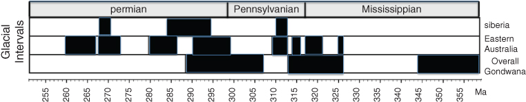
Figure 12.5 Glacial intervals in deep time. Shaded areas are indications of low sea level, inferring the presence of continental ice sheets. The inference of glacial intervals is drawn from sea level evidence (low sea level indicates large volumes of land-based ice).
(Rygel et al. (2008). © American Meteorological Society. Used with permission.)
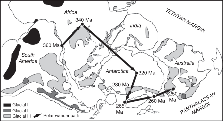
Figure 12.6 An indication of the shifting locations of the South Pole as it passes over portions of Africa, Antarctica, India, and Australia at different times as shown. There are three glacials indicated by the shading in the legend.
(Frank et al. (2008). Reproduced with permission of Geological Society of America.)
12.3.1 Modeling Permian Glacials
Much of climate change over the long term (tens of millions of years) is governed by the greenhouse gas concentrations. This is not an especially interesting aspect of the dynamical behavior of EBMs. The dependence on ![]() concentration is logarithmic (see (2.13) and surrounding discussion). When
concentration is logarithmic (see (2.13) and surrounding discussion). When ![]() concentration doubles, the global temperature will increase by 2–4 K (including feedbacks, and after equilibrium is attained). If the
concentration doubles, the global temperature will increase by 2–4 K (including feedbacks, and after equilibrium is attained). If the ![]() concentration is halved, the temperature will correspondingly decrease by 2–4 K. Interesting problems for EBMs come up when there is a large change in the seasonal cycle, especially when a landmass moves near the pole. When the landmass is large and its center is over the pole, summers will be too hot to initiate or sustain an ice sheet. The action comes when a landmass is near the pole where the mean annual surface temperatures will be low enough for freezing to occur, but again the key is for the summer temperatures to be below freezing. This latter happens if the landmass edge is near the pole or if there is a field of broken landmasses near the pole. The presence of smaller-scale water-covered regions can moderate the summer temperatures, keeping them below freezing. As Pangea breaks up, the chances are good for this to happen.
concentration is halved, the temperature will correspondingly decrease by 2–4 K. Interesting problems for EBMs come up when there is a large change in the seasonal cycle, especially when a landmass moves near the pole. When the landmass is large and its center is over the pole, summers will be too hot to initiate or sustain an ice sheet. The action comes when a landmass is near the pole where the mean annual surface temperatures will be low enough for freezing to occur, but again the key is for the summer temperatures to be below freezing. This latter happens if the landmass edge is near the pole or if there is a field of broken landmasses near the pole. The presence of smaller-scale water-covered regions can moderate the summer temperatures, keeping them below freezing. As Pangea breaks up, the chances are good for this to happen.
A series of studies by Hyde et al. (1990) with a nonlinear (snow/ice–albedo feedback) two-dimensional EBM including a seasonal cycle consider the importance of continental size and positioning with respect to the poles. This study does not include ice-sheet dynamics. There has to be some land near the poles to initiate glaciation. However, the continent covering the poles cannot be too large, otherwise the summers will be too warm to allow snow to build up into an annual ice cover. When the continent is smaller, say 3000 km across, this smaller landmass will allow penetration of the mild maritime summer to suppress the seasonal cycle in the continental interior. Under these conditions, summers will be mild enough (staying below freezing) to allow the snow to build up, eventually leading to an ice field or glacier. The upshot is that the actual geography including shoreline configuration near the pole is important.
An example of conditions that lead to bifurcations (or tipping points) is shown in Figure 12.7 where Crowley and Baum (1993) considered the continental configuration near the South Pole around 300 Ma. In this study, they used the two-dimensional, seasonal EBM similar to the one discussed in Chapter 8. They examined the areas of ice cover for a continuous range of values of the solar luminosity (we have used the more modern term total solar irradiance, TSI ![]() 4) from 327 to 333 W m
4) from 327 to 333 W m![]() . A sharp bifurcation is found as the ice cap suddenly decreases in area.
. A sharp bifurcation is found as the ice cap suddenly decreases in area.

Figure 12.7 Results of a nonlinear 2-D seasonal EBM with ice feedback at 305 Ma. The model was iterated to find the steady solutions. (A) The heavy black line is the outline of the continent (Gondwanaland), the black-shaded areas are locations where data suggest ice sheets during this time. The dotted lines are simulated ice sheets: (a) is for the warmer TSI, and (b) is for an infinitesimally large value of TSI. (B) Shows the area of ice cover as a function of TSI, which is indicated on the abscissa as luminosity. Note the abrupt transition to a smaller ice cap as the TSI passes the bifurcation point.
(Baum and Crowley (1991). Reproduced with permission of Wiley.)
12.4 Glacial Inception on Antarctica
The EBM mechanism for the Antarctic glacial-inception case is based on the geological evidence that Antarctica was once joined to the landmasses of the present Indian subcontinent and present Australia, making the composite continent very “continental” (see Figure 12.8a). Note that the (present) Antarctic continent remains at the pole. Sometime between 80 and 20 Ma the landmass of present India separates from present Antarctica followed by the departure of present Australia (see Figure 12.8b). India proceeds equatorward and across to the collision that results in the present uplift known as the Himalayan Mountains. We are interested in the change leading to a much more maritime Antarctica, wherein the summers at the South Pole would be cooler (see Figure 7.10 and surrounding discussion). As can be seen in Figure 12.9, the summer temperature drops dramatically as Australia disassociates with the Antarctic landmass making each smaller than the combination and much more maritime. The polar temperature falls to about 2.5 ![]() C, but no lower once the influence of the separated twin is no longer important. It is also possible that small fluctuations could cause a jump-over to a larger, more-stable ice cap, see Figure 7.4 and the discussion in Section 7.4.3.
C, but no lower once the influence of the separated twin is no longer important. It is also possible that small fluctuations could cause a jump-over to a larger, more-stable ice cap, see Figure 7.4 and the discussion in Section 7.4.3.
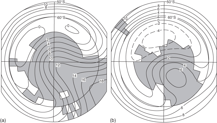
Figure 12.8 (a) Polar view of the SH continental configuration 60 Ma. Solid line contours indicate mid-January temperatures in degree celsius as simulated by the two-dimensional seasonal EBM (North et al., 1983). (b) Same as (a), except 20 Ma. In the interim, Australia shifts away from Antarctica, leaving the latter to be more maritime, thus moderating summer heating at the pole. Poleward of 60 N, the heat capacity of the model's surface is that of sea ice.
(Crowley and North (1988). Reproduced with permission of AAAS.)
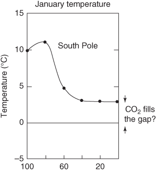
Figure 12.9 Temperatures at the South Pole in mid-summer as a function of time. In this series of simulations, the cooling “saturates” after India completely separates and moves out of an influential distance. The vertical arrows indicate a gap in temperature decrease that should lead to the continental glaciation. DeConto and Pollard (2003) suggest that this gap is closed by the decrease in concentration of  .
.
(Crowley and North (1988). Reproduced with permission of AAAS.)
The EBM-motivated theory uses the “maritimization” of the continent, combined with the seasonal small ice cap instability (Mengel et al., 1988), enabling hot summers in the interior to be mitigated to the freezing point and resulting in “rapid” spread to a stable ice sheet as the main underlying causes of the glacial inception. There are other theories proposing explanations of the Antarctic glacial inception. One of the most cited is that of DeConto and Pollard (2003); they use a simplified GCM called the GENESIS model to simulate the conditions for the glacial inception. They argue in favor of a ![]() decrease from 4 times to about 2 times the present partial pressure
decrease from 4 times to about 2 times the present partial pressure ![]() over a 10 My period. While our argument is crude compared to the detail of these authors, the decline of
over a 10 My period. While our argument is crude compared to the detail of these authors, the decline of ![]() is roughly what our model requires to initiate glaciation. The argument we advance is that our solution is essentially the same as that of DeConto and Pollard. In a later paper, Pollard and DeConto (2005) discuss the small ice cap instability and hysteresis (see Section 7.5) to interpret their low-resolution GCM results. They do not discuss the effect of the recession of the Indian subcontinent and Australia away from Antarctica, as their model simulation is set and conducted after these fixed rearrangements following the separations. The paper by Crowley and North (1988) emphasizing the importance of the seasonality was published well before the recognition of the importance of
is roughly what our model requires to initiate glaciation. The argument we advance is that our solution is essentially the same as that of DeConto and Pollard. In a later paper, Pollard and DeConto (2005) discuss the small ice cap instability and hysteresis (see Section 7.5) to interpret their low-resolution GCM results. They do not discuss the effect of the recession of the Indian subcontinent and Australia away from Antarctica, as their model simulation is set and conducted after these fixed rearrangements following the separations. The paper by Crowley and North (1988) emphasizing the importance of the seasonality was published well before the recognition of the importance of ![]() came to the attention of paleoclimatologists. In fact, both changes in seasonality and the change in
came to the attention of paleoclimatologists. In fact, both changes in seasonality and the change in ![]() are necessary. Carbon cycle models combined with measurements give useful information about
are necessary. Carbon cycle models combined with measurements give useful information about ![]() levels over geological time (references can be found in Zhuang et al., 2014).
levels over geological time (references can be found in Zhuang et al., 2014).
The ![]() O index actually indicates a combination of local temperature (probably at sea bottom) and total ice volume on the land surfaces. Another index taken from the skeletal material (CaCO
O index actually indicates a combination of local temperature (probably at sea bottom) and total ice volume on the land surfaces. Another index taken from the skeletal material (CaCO![]() ) is based on the content of the stable isotope
) is based on the content of the stable isotope ![]() C relative to its normal and much more abundant
C relative to its normal and much more abundant ![]() C and its incremental change of
C and its incremental change of ![]() C index (a measure of the isotopic deviation from normal and far more abundant
C index (a measure of the isotopic deviation from normal and far more abundant ![]() C). This index is a measure of the
C). This index is a measure of the ![]() concentration in the deep ocean. Bender (2013) cites the work of Coxall et al. (2005) who noted that in the neighborhood of the Eocene–Oligocene boundary (34 Ma), the changes in
concentration in the deep ocean. Bender (2013) cites the work of Coxall et al. (2005) who noted that in the neighborhood of the Eocene–Oligocene boundary (34 Ma), the changes in ![]() O and
O and ![]() C are in step, indicating that as the temperature fell, so did the amount of dissolved
C are in step, indicating that as the temperature fell, so did the amount of dissolved ![]() in the oceans. Some back-of-the-envelope estimates in Bender (2013) suggest that a 54 m drop in sea level and a fall of 3–4
in the oceans. Some back-of-the-envelope estimates in Bender (2013) suggest that a 54 m drop in sea level and a fall of 3–4 ![]() C are consistent with the isotope data. These results seem to be in line with the EBM-based theory (seasonal change due to maritimization combined with
C are consistent with the isotope data. These results seem to be in line with the EBM-based theory (seasonal change due to maritimization combined with ![]() decrease), which also agrees with the GCM results of DeConto and Pollard (2003).
decrease), which also agrees with the GCM results of DeConto and Pollard (2003).
Earlier theories of the glacial inception of Antarctica invoke changes in ocean circulation as the Drake Passage is opened. The argument goes that this effect leads to the circumpolar circulation of the Southern Ocean and thus leads to the isolation of Antarctica and therefore its cooling. We believe that the arguments and results presented in Chapter 5, especially those in Section 5.9 and illustrated in Figure 5.10 are pertinent here. In that discussion, the two-mode approximation provides a near-perfect fit to the poleward transport of heat, without reference to any circumpolar current. Simplicity alone suggests that the three components of heat transport (atmospheric sensible heat, latent heat, and oceanic heat) all combine to give a simple form. Just take the NH as a hypothesis and the SH as a confirmation. In light of this, it seems difficult to imagine that the presence or even the intensity of the Circumpolar Current would make a significant difference.
12.5 Glacial Inception on Greenland
The glaciations of Greenland and Antarctica present interesting problems for paleoclimatology and EBMs can contribute to understanding these glaciations (North and Crowley, 1985; Crowley et al., 1986; Crowley and North, 1990). In these studies, covering the times between 80 and 20 My BP, the authors used the rule that summertime maximum temperatures are the key to initiating glaciation. This concept dates back many years (e.g., Milankovitch, 1941). As continents drift over geological time, the maximum value of summer temperature changes depending on latitude and land–sea distributions near the poles. As an example, consider the two configurations shown in Figure 12.10.

Figure 12.10 (a) Polar view of the NH continental configuration 60 My BP. Solid line contours indicate mid-July temperatures in degrees Celsius as simulated by the two-dimensional seasonal EBM (model from North et al., 1983). Opening of the land bridge connecting Greenland and Europe results in a distortion of the freezing line (0  C) as shown by the dotted line. (b) Same as (a), except this is for 40 My BP. In the interim, Greenland shifts poleward and it becomes more maritime. Poleward of 60
 N, the heat capacity of the model's surface is that of sea ice.
(Crowley and North (1988). Reproduced with permission of AAAS.)
Figures 12.10a and 12.10b show the continental configurations for 60 and 40 Ma, respectively. The solid lines depict the contours of the mid-July temperatures as computed from the EBM (North et al., 1983). In both (a) and (b), poleward of 60![]() N, North et al. (1983) used the value of sea ice over the ocean-covered areas (
N, North et al. (1983) used the value of sea ice over the ocean-covered areas (![]() is taken to be part way between land and ocean values, to take into account puddling and leads). Figure 12.11a shows the simulated mid-July temperature changes in Greenland, in which we see a definite cooling in mid-summer in the interior of Greenland over the 20 My change. Figure 12.11b shows the seasonal cycle of the mid-Greenland surface temperature for various times in the geological past, 100 Ma to the present. Two factors clearly cause the mid-summer temperatures to decline: (i) Greenland's movement toward the poles causes the mean annual temperature to fall; (ii) the seasonal cycle amplitude is diminished because Greenland has become more maritime.
is taken to be part way between land and ocean values, to take into account puddling and leads). Figure 12.11a shows the simulated mid-July temperature changes in Greenland, in which we see a definite cooling in mid-summer in the interior of Greenland over the 20 My change. Figure 12.11b shows the seasonal cycle of the mid-Greenland surface temperature for various times in the geological past, 100 Ma to the present. Two factors clearly cause the mid-summer temperatures to decline: (i) Greenland's movement toward the poles causes the mean annual temperature to fall; (ii) the seasonal cycle amplitude is diminished because Greenland has become more maritime.
Figure 12.11b suggests that at about 15 My, BP the mid-summer temperatures fall below freezing (see also Figure 12.12). If we combine this finding with the small ice-cap instability argument, we can envision that at this point, a small ice cap is not possible; hence, there must be a transition to a finite-sized ice cap. Such an ice cap would cover all of Greenland. The theory is very simple, and compelling because it gets the timing right and it calls for a continent-sized ice sheet.

Figure 12.11 (a) Mid-July temperature differences between 60 and 40 Ma as simulated by the 2-D seasonal EBM, North et al. (1983). (b) The seasonal cycle of mid-Greenland for various times 100 My to the present. Two features are apparent: (i) the mean annual temperature is lowered by the shift, (ii) the seasonal cycle is cut by nearly a factor of 2. Both effects tend to lower mid-summer temperatures.
(Crowley and North (1988). Reproduced with permission of AAAS.)
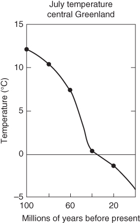
Figure 12.12 Mid-summer temperatures as simulated with the 2-D seasonal EBM as a function of time (in Ma).
(Crowley and North (1988). Reproduced with permission of AAAS.)
12.6 Pleistocene Glaciations and Milankovitch
Lisiecki and Raymo (2005) used a “stack” of 57 cores well distributed over the ocean floor to examine ![]() O isotope variations in benthic2 Foraminifera3 to study global changes in ice volume and temperature over the last few million years. They found that roughly 5 million years ago, the ice volume on the planet began making irregular oscillations with a period close to 41 ky (see Figure 12.13). By 2 million years ago, the oscillations became more regular at this same period. Figure 12.13 shows the results of their study which combined 57 globally distributed seafloor cores of data based on
O isotope variations in benthic2 Foraminifera3 to study global changes in ice volume and temperature over the last few million years. They found that roughly 5 million years ago, the ice volume on the planet began making irregular oscillations with a period close to 41 ky (see Figure 12.13). By 2 million years ago, the oscillations became more regular at this same period. Figure 12.13 shows the results of their study which combined 57 globally distributed seafloor cores of data based on ![]() O from bottom-dwelling microspecies (benthic foraminifera). The signal is particularly strong given that so many samples were averaged together. Figure 12.14 shows the spectral density of the record of ice volume–temperature.4 The record of ice volume being inferred from such data has a long history. There are now many independent corroborating pieces of evidence such as that from ice cores,5 blown dust (loess6) deposits whose timings match well with deep-sea core data (Bender, 2013; Bradley, 2015).
O from bottom-dwelling microspecies (benthic foraminifera). The signal is particularly strong given that so many samples were averaged together. Figure 12.14 shows the spectral density of the record of ice volume–temperature.4 The record of ice volume being inferred from such data has a long history. There are now many independent corroborating pieces of evidence such as that from ice cores,5 blown dust (loess6) deposits whose timings match well with deep-sea core data (Bender, 2013; Bradley, 2015).
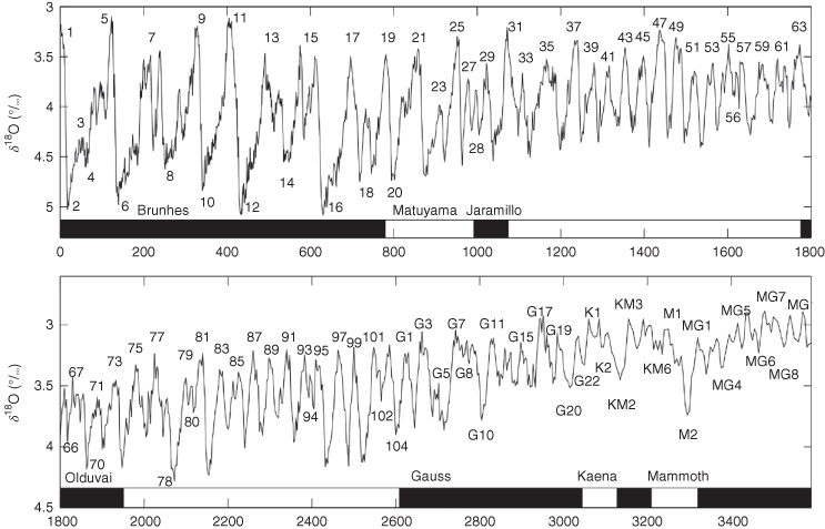
Figure 12.13 Time series of data from 57 globally distributed  O taken from the shells of bottom-dwelling microspecies (benthic foraminifera). The numbers above and below the peaks and valleys indicate the stage-name of the local extreme event.
(Lisiecki and Raymo (2005). Reproduced with permission of Wiley.)
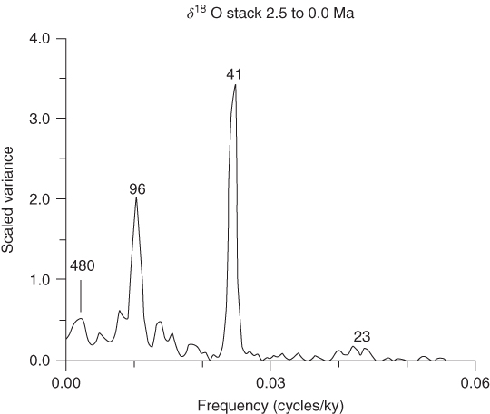
Figure 12.14 Spectra from a “stack” (similar to an ensemble average) of globally distributed seafloor cores of data on  O. The data in this figure come from 2.5 Ma to the present. Note the strong peaks at 41 ky (obliquity), 23 ky (precession) as well as 480 and 96 ky (eccentricity).
(Hartmann (1994). Reproduced with permission of Academic Press.)
The Milankovitch7 theory of the ice ages (Milankovitch, 1998)8 links the nearly periodic changes in the orbital parameters of the Earth's motion around the Sun to the periodic glaciations. It received little attention until the sea cores began to reveal the clear indication of periodicity of the glaciations, first from Emiliani (1958), culminating with the Hayes et al. (1976) paper that directly compared the sea core data with the orbital element variations based on celestial mechanics, essentially confirming the Milankovitch mechanism as the “pacemaker” of the ice ages. Figure 12.15 shows the temporal variation of the orbital elements (eccentricity, obliquity, and precession of the equinoxes) based on calculations conducted by Berger (1978). Figure12.15 shows spectra of the insolation at different latitudes and times of year, based upon a time series of calculated insolation values over the last 468 000 years. Figure 12.15a shows the spectra of the quantity ![]() , where
, where ![]() is eccentricity and
is eccentricity and ![]() is the phase of perihelion. Here, the contribution from the obliquity (peaked at period 41 ky) is represented by the solid line, while that of the precession (periods of 23 and 19 ky) are in dotted lines.
is the phase of perihelion. Here, the contribution from the obliquity (peaked at period 41 ky) is represented by the solid line, while that of the precession (periods of 23 and 19 ky) are in dotted lines.
Figure 12.16 shows the spectra from actual data. Figure 12.16b shows the percentage of Cycladophora davisiana over all other radiolaria9 in the time-interval samples. The presence of species relative to other forms of radiolaria is known to indicate the temperature near Antarctica.

Figure 12.15 Solar insolation at different latitudes and seasons calculated over the last 468 000 years. (a) The parameter  , where
  is eccentricity,
  is the phase of perihelion. (b) Insolation at 55
 S in winter. (c) The insolation at 60
 N in summer. The peak frequencies are at period 41 ky (obliquity) and 23 ky together with 19 ky for precession. Figure from Hayes et al. (1976).
(©Amer. Assoc. Advance. Sci., with permission.)
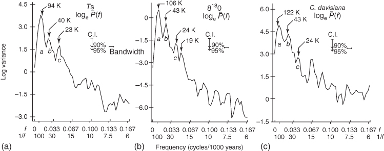
Figure 12.16 Log spectra from two subantarctic deep-sea cores. (a) The surface temperature estimated from radiolarian assemblages. (b)  O. (c) The percentage of C. davisiana relative to all other radiolaria.
(Hayes et al. (1976). Reproduced with permission of AAAS.)
12.6.1 EBMs in the Pleistocene: Short's Filter
The study of EBMs leads to some interesting results for the Pleistocene. We start with the 2-D seasonal model of North et al. (1983) (see also North and Crowley, 1985). The model was run with the present TSI, then small percentage changes in the TSI were used. Ice cover was prescribed when the summer temperature fell below freezing. The model was iterated until a steady state was found. Figure 12.17 shows that a bifurcation occurs at a value between ![]() 1 and
1 and ![]() 2
2 ![]() C. Below this value, the “ice sheet” extends completely across the Arctic Ocean and includes Alaska and much of western Canada, even some of Siberia. This “glaciation” is asymmetric between the Eastern and Western hemispheres—there is more ice cover in the Western hemisphere. But the big ice sheet does not resemble the Laurentide Ice Sheet much. There could be some problems with the model perhaps due to its poor spatial resolution. Experience with previous nonlinear, one-dimensional models with ice caps (Chapter 7 and especially Figures 7.10 and 7.12, both taken from Mengel et al., 1988) suggest that the transition to extensive ice cover might be rather rapid.
C. Below this value, the “ice sheet” extends completely across the Arctic Ocean and includes Alaska and much of western Canada, even some of Siberia. This “glaciation” is asymmetric between the Eastern and Western hemispheres—there is more ice cover in the Western hemisphere. But the big ice sheet does not resemble the Laurentide Ice Sheet much. There could be some problems with the model perhaps due to its poor spatial resolution. Experience with previous nonlinear, one-dimensional models with ice caps (Chapter 7 and especially Figures 7.10 and 7.12, both taken from Mengel et al., 1988) suggest that the transition to extensive ice cover might be rather rapid.
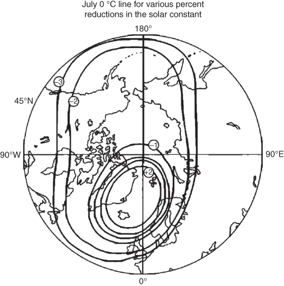
Figure 12.17 Morphology of the mid-July 0  C isotherm for various percentage changes in the total solar irradiance. Contours are for every 1% from +2 to
  3.
3.
(North et al. (1983). © American Meteorological Society. Used with permission.)
A comprehensive chapter by Short et al. (1991) shows a number of linear responses to orbital element changes by the 2-D seasonal model (North et al., 1983) discussed in Chapter 8. In this section, we present results from this paper. As referred to in the title of the paper, the responses are the result of filtering the changes in orbital element forcing through the model being thought of as a “filter.” It is useful to note that the model is solved for its mean annual solution, its annual harmonic solution, and its semiannual solution. Then these Fourier components are composed into the complete solution for the seasonal cycle of the temperature field. But it is interesting to examine the effect on the Fourier components directly both in the insolation and in the responses.
First consider the latitude dependence of the forcing (perturbation of the insolation components). Figure 12.18 shows how the insolation as function of latitude changes for extreme values of the obliquity (a) and for the precession varying from perihelion to aphelion (b). It is interesting that the insolation in both (a) and (b) show that some harmonics of the insolation dip to negative values near the equator.
Next consider the geographical distribution of the response in maximum NH summer temperatures (![]() C) due to a change in obliquity from its known extremes 22.1
C) due to a change in obliquity from its known extremes 22.1![]() (solid) to 24.4
(solid) to 24.4![]() (see Figure 12.19). In this case, the eccentricity is set to zero. The continents are shown with blocklike edges to emphasize the course resolution of the model. The tropical response in this figure shows a negative response (180
(see Figure 12.19). In this case, the eccentricity is set to zero. The continents are shown with blocklike edges to emphasize the course resolution of the model. The tropical response in this figure shows a negative response (180![]() out of phase with the extratropical response). Short et al. (1991) point out that this is in agreement with results of core RC24-30 taken in the tropical Atlantic (Imbrie et al., 1992).
out of phase with the extratropical response). Short et al. (1991) point out that this is in agreement with results of core RC24-30 taken in the tropical Atlantic (Imbrie et al., 1992).
Figure 12.20 shows the response pattern of northern summer temperatures as the summer solstice moves from aphelion to perihelion. Figure 12.21 combines the difference of extremes for obliquity and maximum eccentricity (0.06). The Southern Hemisphere is also depicted at summer solstice by combining data from the two hemispheres at six-month intervals into one map.

Figure 12.18 (a) The latitude dependence of the insolation for obliquity = 24.4 to 22.1
 (dashed), for the Fourier components, first harmonic, and second harmonic. The eccentricity is set to zero. (b) The same but for precession extrema for eccentricity = 0.06.
(Short et al. (1991). Reproduced with permission of Elsevier.)
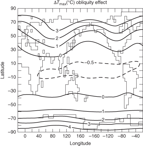
Figure 12.19 The obliquity effect. Geographic pattern of the change in maximum summer temperature as the obliquity changes from 22.1 (solid) to 24.4
 .
.
(Short et al. (1991). Reproduced with permission of Elsevier.)
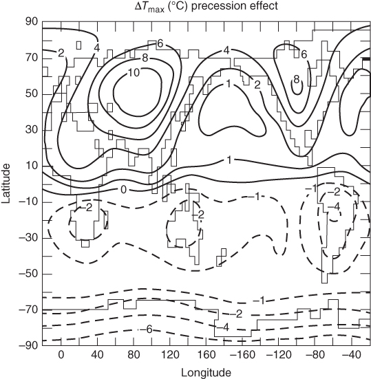
Figure 12.20 The precession effect. Geographic pattern of the change in maximum summer temperature as summer solstice moves from aphelion to perihelion with eccentricity at its maximum value, 0.06 and the obliquity is the present value, 23.25 .
.
(Short et al. (1991). Reproduced with permission of Elsevier.)

Figure 12.21 Combined effect. Geographic pattern of the change in maximum summer temperature as northern summer solstice moves from aphelion to perihelion with eccentricity at its maximum value, 0.06 and the obliquity is the present value, 24.4 . In this figure, both hemispheres are shown in summer by combining data from runs of each.
(Short et al. (1991). Reproduced with permission of Elsevier.)
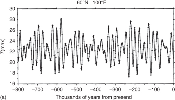
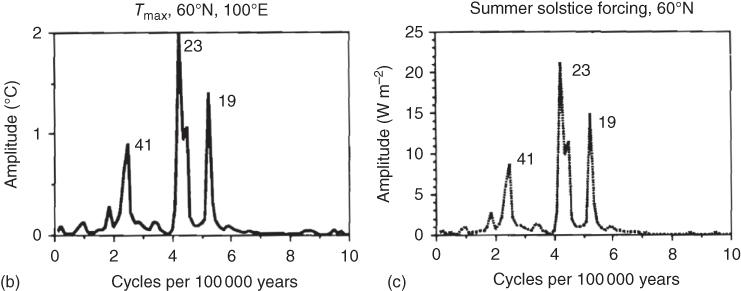
Figure 12.22 (a) Time series of the maximum summer temperature response at 60 N, 100
 E (north central Asia) as simulated by the model after running for the last 800 000 years. From Short et al. (1991). (b) The amplitude spectrum of
  , the time series shown in panel (a). (c) The amplitude forcing for summer at 60
 N. Major peaks are labeled with the periodicity in thousands of years.

Figure 12.23 (a) Fourier amplitude spectrum of the time series of maximum summer temperature response at 50 N, 30
N, 30 W (north Atlantic), as simulated by the model after running for the last 800 000 years. (b) The amplitude spectrum of orbital forcing for summer at 50
 N. Major peaks are labeled with the periodicity in thousands of years. Figure from Short et al. (1991).
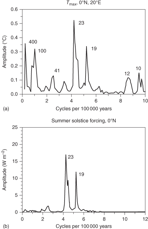
Figure 12.24 (a) Fourier amplitude spectrum of the time series of maximum summer temperature response at 0 N, 20
N, 20 E (equatorial Atlantic) as simulated by the model after running for the last 800 000 years. (b) The amplitude spectrum of orbital forcing for summer at 60
 N. Major peaks are labeled with the periodicity in thousands of years. Figure from Short et al. (1991).

Figure 12.25 The seasonal cycle of sea surface temperature simulated at 0 N, 20
N, 20 E for epoch 98, 94, 90, 86 ka. The abscissa is the number days after winter solstice. The figure shows the simulated temperature at the equator in the Atlantic Ocean. There are two local maxima at 86 ky (crosses) as the Sun passes overhead at the equator at both vernal and autumnal equinox. As time passes through the precession cycle, the two maxima become only one, either in the spring or in the autumn. This effect leads to two maximum temperatures over the 22-year cycle. The result is a peak at twice the frequency or half the period of the forcing (
 ky in the previous figure). Figure from Short et al. (1991).
Next are considerations of how the changes in insolation are filtered into the thermal responses especially over oceans where deep-sea cores are collected. We are always interested in the maximum summer temperature in this series of simulations. While the summer temperature field is a linear response to the forcing, the maximum summer temperature is not a linear function of the forcing because finding the maximum is the result of finding the root of the equation ![]() after we have found
after we have found ![]() , where
, where ![]() is the
is the ![]() and
and ![]() is the time after winter solstice in the repeating seasonal cycle. In the center, the great continent of Asia where the relaxation timescale is much less than a year, the response (a) mirrors that of the forcing (b) at each of the orbital signals (see Figure 12.22).
is the time after winter solstice in the repeating seasonal cycle. In the center, the great continent of Asia where the relaxation timescale is much less than a year, the response (a) mirrors that of the forcing (b) at each of the orbital signals (see Figure 12.22).
As we look at different points in the Atlantic, the response as filtered from the forcing (and the maximum found) presents different results from points in the center of a large continental landmass. Figures 12.22 and 12.23 focused on the north Atlantic shows the time series and amplitude spectra of the maximum summer temperature and the insolation. Here we see strong peaks at the obliquity and precession periods, but also several low-frequency peaks. These are related to the eccentricity and its effect on the other orbital elements.
In equatorial Atlantic (0![]() N, 30
N, 30![]() E), as seen in Figure 12.24, the obliquity signal is weak, but the eccentricity frequencies corresponding to periods of 400 and 100 ky are very strong. Note also a first harmonic of the two precession frequencies (periods of
E), as seen in Figure 12.24, the obliquity signal is weak, but the eccentricity frequencies corresponding to periods of 400 and 100 ky are very strong. Note also a first harmonic of the two precession frequencies (periods of ![]() and 10 ky). These harmonics are explained in Figure 12.25 (see also Short and Mengel, 1986). Figure 12.25 shows the response as function of lag (days) after the winter solstice. At 86 ky, the temperature curve (indicated by +s) is symmetric about the summer solstice as the Sun passes over the equator twice during the year. There are two maxima of equal magnitude at this time. Then a quarter of the precession cycle later at 90 ky (indicated by
and 10 ky). These harmonics are explained in Figure 12.25 (see also Short and Mengel, 1986). Figure 12.25 shows the response as function of lag (days) after the winter solstice. At 86 ky, the temperature curve (indicated by +s) is symmetric about the summer solstice as the Sun passes over the equator twice during the year. There are two maxima of equal magnitude at this time. Then a quarter of the precession cycle later at 90 ky (indicated by ![]() s), there is one absolute maximum. Next consider 94 ky (indicated by
s), there is one absolute maximum. Next consider 94 ky (indicated by ![]() s), when there are two (nearly) equal maxima. Finally, in the cycle at 98 ky (indicated by △s), there is a single global maximum. This sequence shows that there are two global maxima occurring at a separation of about one half of the precession period. Finding the absolute maxima as a function lag in the seasonal cycle is a nonlinear procedure from the direct forcing amplitude: hence, the first harmonic of the forcing.
s), when there are two (nearly) equal maxima. Finally, in the cycle at 98 ky (indicated by △s), there is a single global maximum. This sequence shows that there are two global maxima occurring at a separation of about one half of the precession period. Finding the absolute maxima as a function lag in the seasonal cycle is a nonlinear procedure from the direct forcing amplitude: hence, the first harmonic of the forcing.
Before moving away from spectra, we draw attention to the latitude dependence of observed spectra. Figure 12.26 shows two spectral densities of temperatures estimated from microfossils along the Mid-Atlantic Ridge. The right-most spectrum from a latitude of 41![]() shows a prominent peak at 23 ky and the leftmost shows a similar spectrum but taken at 54
shows a prominent peak at 23 ky and the leftmost shows a similar spectrum but taken at 54![]() N, where the 23 ky peak has disappeared and a peak at 41 ky appears prominently. This is close to what the 2-D model would suggest. As we leave Short's work, we see how the linear model is able to produce spectra comparable to our expectation and even some data in the middle and lower latitudes. Moreover, the nonlinearity of the maximum summer temperatures as driven by linear responses of the temperature field invites the possibility of under- and overtones appear in the spectra along with evidence of the eccentricity cycles.
N, where the 23 ky peak has disappeared and a peak at 41 ky appears prominently. This is close to what the 2-D model would suggest. As we leave Short's work, we see how the linear model is able to produce spectra comparable to our expectation and even some data in the middle and lower latitudes. Moreover, the nonlinearity of the maximum summer temperatures as driven by linear responses of the temperature field invites the possibility of under- and overtones appear in the spectra along with evidence of the eccentricity cycles.

Figure 12.26 The spectral variance densities of the mid-Atlantic sea cores: K708-7 at 54 N and V30-97 at 41
 N. Note that the more tropical core shows a strong peak at period 23 ky and the more polar core has its peak at 41 ky, both having a strong variance at 100 ky. Modified from Ruddiman and McIntyre (1984), Geol. Soc. Amer. Bull. 95, 381–396.
(© Geological Society of America, with permission).
An interesting set of paleoclimatological experiments with the linear seasonal 2-D EBM were recently conducted by Zhuang (private communication, 2015). He employed the same physical model as was used in North et al. (1983), but as modified by Stevens who used a finite-difference numerical scheme based on multigrid relaxation as discussed in Bowman and Huang (1991), Huang and Bowman (1992), Stevens and North (1996). No parameter changes were employed in his work. Among his experiments were the following cases shown in Figure 12.27. Panel (a) shows a simulation of the linear (no ice feedback) model wherein the full Last Glacial Maximum (LGM) were employed, including the orbital parameters, the concentration of ![]() , and the placement of ice in the Laurentide Ice Sheet, the Greenland Ice Sheet, and the Fenno-Scandian Ice Sheet. As usual, no topography and no dynamical ice volume model were introduced in the EBM. It can be seen that the summertime 5
, and the placement of ice in the Laurentide Ice Sheet, the Greenland Ice Sheet, and the Fenno-Scandian Ice Sheet. As usual, no topography and no dynamical ice volume model were introduced in the EBM. It can be seen that the summertime 5 ![]() C line hugs the equatorward edge of the ice sheet on both continents. While he did not iterate the solution to include the ice–albedo feedback, it appears that this would be a solution if the ice line were to be close to the 5
C line hugs the equatorward edge of the ice sheet on both continents. While he did not iterate the solution to include the ice–albedo feedback, it appears that this would be a solution if the ice line were to be close to the 5 ![]() C line. Figure 12.27b shows the simulated temperature (linear model) when the ice albedo of the Laurentide Ice Sheet is removed and replaced by bare land, while the concentration of
C line. Figure 12.27b shows the simulated temperature (linear model) when the ice albedo of the Laurentide Ice Sheet is removed and replaced by bare land, while the concentration of ![]() and the orbital elements were unaltered from their LGM settings. As the figure shows, the 5
and the orbital elements were unaltered from their LGM settings. As the figure shows, the 5 ![]() C line jumps to leave only Greenland and northwestern Eurasia with ice cover. It appears that the ice albedo is dominant over the other conditions, which seem to play a rather minor role. This is a rather puzzling result. It suggests that there are equilibrium solutions for the big ice sheet and for a small one. An attractive possibility is that if the ice is placed there it will stay. If remove it will remain removed. This may be a kind of neutral stability. Perhaps a large fluctuation could make it jump, aided by the orbital forcing. Another result that has been known for some time is that the orbital perturbation alone is not enough to start an ice sheet in North America. Might a large fluctuation do the trick? We leave this to the imagination of our readers.
C line jumps to leave only Greenland and northwestern Eurasia with ice cover. It appears that the ice albedo is dominant over the other conditions, which seem to play a rather minor role. This is a rather puzzling result. It suggests that there are equilibrium solutions for the big ice sheet and for a small one. An attractive possibility is that if the ice is placed there it will stay. If remove it will remain removed. This may be a kind of neutral stability. Perhaps a large fluctuation could make it jump, aided by the orbital forcing. Another result that has been known for some time is that the orbital perturbation alone is not enough to start an ice sheet in North America. Might a large fluctuation do the trick? We leave this to the imagination of our readers.
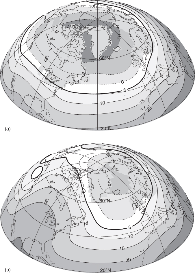
Figure 12.27 Results of simulation with the linear seasonal 2-D EBM (provided privately by Zhuang). (a) The summer average surface temperature with prescribed orbital configuration,  concentration, and land-based ice in North America (Laurentide), Greenland, and Europe (Fenno-Scandian) at the Last Glacial Maximum (LGM) 20 000 year BP. (b) The same except that the prescribed ice sheet in North America is removed. No other changes from LGM conditions were made.
(Courtesy Dr. Kelin Zhuang.)
12.6.2 Last Interglacial
Figure 12.28 shows a time series going back to 420 ka from the ice core data derived from the Vostok site in Antarctica (Petit et al., 2001). Estimates of temperature departures from a modern long-term average are plotted versus time, increasing from right to left. The last interglacial is the peak between roughly 110 and 140 ka. Other information from this core including other proxies, ![]() concentrations, and spectral estimates can be found in Petit et al. (1999).
concentrations, and spectral estimates can be found in Petit et al. (1999).
Crowley and Kim (1994) employed the two-dimensional, seasonal EBM (described in Chapter 8) to study temperatures and inferred estimates of sea level during the last interglacial (LIG). They found model indications of 3–![]() C July (mid-summer) increases at high latitudes from 140 to 130 ka. In these simulations, they kept
C July (mid-summer) increases at high latitudes from 140 to 130 ka. In these simulations, they kept ![]() fixed but included the forcing from obliquity and precession changes over that period. The three sites are (75
fixed but included the forcing from obliquity and precession changes over that period. The three sites are (75![]() N, 120
N, 120![]() W), Northern Canada, (75
W), Northern Canada, (75![]() N, 30
N, 30![]() E) Arctic Ocean north of Scandinavia, and (45
E) Arctic Ocean north of Scandinavia, and (45![]() N, 90
N, 90![]() W), US Canadian border near Lake Superior. They note the following:
W), US Canadian border near Lake Superior. They note the following:
Although it is at the same latitude as the Barents Sea site, peak warming at the Canadian Arctic site occurred 4000 years later. This response reflects the greater importance of the precession-controlled continentality effect on the Canadian site. However, all sites were warmer than they are now by 130 000 years ago.
They suggest that the Milankovitch forcing might be responsible for the decaying ice sheet (see Figure 12.29).
The problem of temperature and sea level (ice volume) during the LIG has recently received attention especially because of its similarity to the present interglacial. Some studies suggest that sea level might have been much higher during the LIG.

Figure 12.28 Time series of temperature estimates (departures from recent time average  C) from the Vostok ice core based on
  isotope departures. The Holocene, Last Glacial Maximum (LGM), and the Last Interglacial are indicated. The Last Interglacial is nominally the period between 130 and 110 ka. The three sites are (75
 N, 120
 W) Northern Canada, (75
 N, 30
N, 30 E) Arctic Ocean north of Scandinavia, and (45
 N, 90
N, 90 W) US Canadian border near Lake Superior. (NASA.)
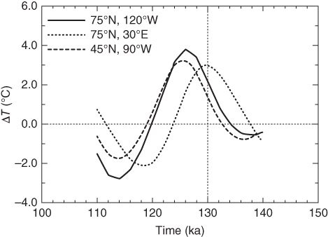
Figure 12.29 Time series of model simulations of departures of July temperatures from present at three locations over the period 140 to 110 ka. Figure from Crowley and Kim (1994).
(©Amer. Assoc. Advance. Sci., with permission.)
12.6.3 EBMs and Ice Volume
Since the two-dimensional-seasonal EBM (North et al., 1983) simulates the seasonal cycle surface temperature well to first order, it was natural that Peltier and colleagues use it in their modeling of the glacial–interglacial cycles of the Pleistocene (DeBlonde and Peltier, 1991; Hyde and Peltier, 1987). Also, Pollard (1982) has tried including an ice model to an EBM comparable to the beachball model (see Section 8.1). Others, including Paillard (2001), tried combining ice models to EBMs. As noted by Huybers and Wunsch (1994), this combination always leads to a number of new tunable parameters, as there are only eight or so glaciations at the 100 ky timescale. The problem of tuning comes up immediately, as one tries to model glacial growth by inserting precipitation in the form of snow. But this is only the one of the problems encountered as one contemplates the flow and decay of ice sheets. This is not to discourage experimentation wherein much might be learned, but it is to recognize that this is a very big step fraught with potential errors of overfitting.
Crowley and Hyde (2008) re-plotted the Lisiecki and Raymo data in a way that emphasizes the increase of amplitude and the lower frequencies of the fluctuations as a function of time. They note the striking resemblance between Figure 2.10 and Figure 12.30 that have been reproduced from Crowley and North (1988). Crowley and Hyde (2008) argue that a series of threshold crossings are in progress. First is a small ice sheet in North America, then a transition to a larger one. Next is a smaller ice cover in northeastern Europe. Finally, to come is a large ice sheet in Eurasia. Their model goes beyond the simple EBMs of this book in employing a dynamical ice sheet.

Figure 12.30 The  O record as replotted by Crowley and Hyde (2008). These authors argue that as the planet cools during the last 3.0 Ma the amplitude of the fluctuations increases. Each new oscillation seems to have a larger amplitude and a lower frequency—perhaps an indicator of another bifurcation coming up.
(Crowley and Hyde (2008). Reproduced with permission of Nature.)
An unsolved puzzle is the transition from the so-called 41 ky world to the 100 ky world. This is clearly shown in Figures 12.13 and 12.30 wherein the peaks in global ice volume suddenly change from a dominant obliquity forcing to that associated with the less well understood 100 ky forcing. Interesting attempts at explaining the transition are reviewed in Raymo and Huybers (2008). One mystery is: Why are not the 21 ky peaks evident in the “41 ky world?” Raymo notes that the precession forcing is antisymmetric between the hemispheres and she posits the ice volume forcing may be canceling. Huybers has been interested in the possibility of integrating the insolation over the entire summer season, whose length changes with the precession phase and is modulated by the eccentricity.
12.6.4 What Can Be Done without Ice Volume
Our use of EBMs in paleoclimatology has been to partially answer questions about the inception of glaciation as in Sections 12.4 and 12.5. EBMs might be able to address these issues without any new adjustable parameters. This is as opposed to trying to map the detailed time series in order to compare with a corresponding time series of data. We are guided by the results shown in Figure 7.10 where a latitude-only seasonal EBM was run with a disklike continent centered at the pole. This simulation shows how as a threshold of some control parameter is crossed there is a qualitatively different steady state. Figure 7.12 shows that as the threshold is crossed, it may take tens if not hundreds of years to adjust to the new steady state. The long adjustment time is a result of the nonlinear snow-albedo effect. This time as illustrated in that figure is sensitively dependent on the initial conditions in the problem. This is done without any noise forcing in the problem. One wonders how this bizarre behavior would be affected by background noise as in Chapter 9. Figure 7.14 shows another case where a zonal band of land replaces the pole-centered disk. In this band-of-land geography there are two thresholds. This kind of simulation is tricky because one must be very careful to use high latitudinal resolution. One cannot help but wonder what happens if there is longitudinal dependence in this nonlinear seasonal EBM. And what if noise is included? Might there be quasi-periodic jumping? Some seasonal simulations of two dimensional, seasonal EBMs including nonlinear snow feedback and with realistic and idealized two-dimensional geography (in their case, the late Permian geography) have been conducted by Baum and Crowley (1991). The two-dimensional seasonal simulations seem to confirm the one-dimensional works of Mengel et al. (1988) and Lin and North (1990), and Huang and Bowman (1992) that bifurcations exist when (not-too-large, or appropriately fragmented) landmasses lie near or at the poles when forced by a seasonal cycle with an interactive snowline. Then Crowley et al. (1994) used to Genesis GCM to investigate the effect. They showed a comparison between the EBM and the GCM results. The GCM seems to confirm the bifurcationand the corresponding catastrophic change in ice cover as the TSI ![]() is varied.
is varied.
Notes for Further Reading
Bradley (2015) has written the most comprehensive book on the climate of the last few million years. It is especially good on the observational evidence including its promise and its limitations. Bender (2013) has written an nice book that covers a lot of ground from the Precambrian to theHolocene and written by an expert especially on the isotope chemistry. Another recent well written book with lots of references is that of Summerhayes (2015), a marine geologist. Bender's book in the Princeton University Press series is well written and up to date. The field is changing rapidly and sadly the book by Crowley and North (1988) is out of print and mostly out of date.
There is not much direct evidence of ![]() changes over the long timescale spanning the Phanerozoic (last 540 Ma), hence, models have to be employed to make inferences about the record of this greenhouse gas. The book by Berner (2004) explains the many considerations that go into such a model with some details about the processes involved. This book also discusses the evolution of
changes over the long timescale spanning the Phanerozoic (last 540 Ma), hence, models have to be employed to make inferences about the record of this greenhouse gas. The book by Berner (2004) explains the many considerations that go into such a model with some details about the processes involved. This book also discusses the evolution of ![]() . An excellent recent book on paleoclimatology including many historical notes written by a marine geologist is by Summerhayes (2015).
. An excellent recent book on paleoclimatology including many historical notes written by a marine geologist is by Summerhayes (2015).
As this manuscript was being submitted for publication, a special issue of the periodical Past Global Changes Magazine, 24, No. 1, August 2016, arrived. This happens to be a special issue on tipping points, which is of interest to readers of Chapter 12 as well as several others that cover bifurcations in the solutions of EBMs.
Exercises
12.1 For this exercise, use the program called milank.f, which computes the orbital parameters (obliquity, eccentricity, perihelion angle, precession index) based on the Milankovitch theory. (This program is available at the author's (KYK) website.)
- a. Calculate the orbital parameters for the past 1000 ky at intervals of 1 ky. Plot the four orbital parameters.
- b. On the basis of spectral analysis, determine the major periodicities in the time series of obliquity, eccentricity, and precession.
12.2 The magnitude of solar irradiance varies according to the distance between the Sun and the Earth. The amount of solar irradiance is given by

where
 is the mean solar irradiance and
  is the true anomaly.10
- a. Calculate the solar irradiance as a function of
 for three different values of eccentricity:
  , and 0.04.
 - b. What would be the percentage change in the solar constant between the perihelion and aphelion when the eccentricity is 0.04?
- a. Calculate the solar irradiance as a function of
12.3 For this exercise, use “insol.f” which computes insolation distribution function for given orbital parameters. (This program can be found at the author's website.)
- a. Run the program to calculate the insolation distribution function for the present orbital configuration and that at 15 ky BP (before present). Hint: The insolation program requires orbital parameters, which can be calculated by executing milank.f program.
- b. Describe the difference in insolation between the two time periods. Explain why. Describe what you would expect in the NH and SH polar regions.